Attention concept overview
Building on this foundation, think of an attention mechanism as a dynamic routing layer that lets the model decide which parts of the input deserve computation and which can be ignored. In the first 100 words we’ll anchor core terms: attention mechanism and self-attention are the primitives that replaced strict recurrence in many modern models. Rather than processing tokens strictly in order, attention scores encode relevance between positions so you can compute context vectors as weighted sums. This reframes sequence modeling from “step-by-step” to “compare-and-aggregate,” which unlocks parallelism and richer contextual reasoning.
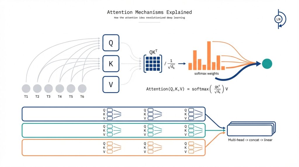
At its core, attention maps three concepts—queries, keys, and values—into a similarity-weighted read operation. How do you compute attention efficiently? The common pattern is scaled dot-product attention: take Q·K^T, divide by sqrt(d_k) to stabilize gradients, apply softmax across keys to get weights, and multiply those weights by V to produce the contextualized output. That simple pipeline converts pairwise affinities into continuous attention distributions, and it is numerically stable and highly optimized on GPUs because it reduces to large matrix multiplications.
Self-attention is the special case where queries, keys, and values all come from the same sequence, enabling each position to attend to every other position. We use multi-head attention to let the model attend with different representation subspaces in parallel: split embedding channels into H heads, run independent attention for each head, then concatenate and project back. For example, in machine translation a single head might capture short-range syntactic dependencies while another tracks long-range subject–verb agreement; combining them yields a richer encoding than a single monolithic attention map.
Practical constraints shape how we apply attention in real systems: the naive attention operation has O(n^2) time and space complexity with sequence length n, so long documents and high-resolution images become expensive. To handle this, engineering teams use strategies like chunking into windows, applying sparse or locality-sensitive attention, or adopting linearized attention kernels that approximate softmax. For autoregressive generation you also need causal masking to prevent peeking at future tokens; for padding and batching you apply attention masks so compute focuses only on valid positions.
When you implement attention, treat matrix efficiency and numerical stability as first-class concerns. Use batched GEMM (general matrix multiply) for Q·K^T and attention-weighted V to leverage hardware acceleration; scale by sqrt(d_k) before softmax to avoid vanishing gradients; and apply dropout to attention weights during training to regularize head co-adaptation. In practice your tensors will look like (B, H, T, D_h) for queries/keys/values where B is batch, H heads, T tokens, and D_h = d_model/H; keeping these consistent simplifies fused kernel integration and mixed-precision training.
Where does attention shine in real projects and when should you avoid it? Choose attention when you need flexible, global context—transformer-style architectures dominate tasks from translation and summarization to code completion and vision with patch-based models. However, on very long inputs or resource-constrained edge devices, consider hybrid approaches that combine local convolutions or recurrence with sparse attention to reduce cost. Taking this concept further, next we’ll examine how attention composes into the Transformer block and the practical engineering patterns—layer normalization, residual paths, and head pruning—that make production models efficient and robust.
Why attention matters
Building on this foundation, the practical reason we care about an attention mechanism is that it changes how models allocate computation and represent context. How do you make a model weigh useful context over noise when input length and semantics vary wildly? Attention gives you a differentiable, data-driven routing layer: queries score keys, attention weights select values, and the model learns which positions matter for each prediction. By front-loading “attention” and “self-attention” in your mental model, you start treating sequence modeling as dynamic read operations instead of fixed-step transforms, which immediately affects architecture, debugging, and deployment choices.
The most visible payoff is modeling long-range dependencies without enforced recurrence. Where a recurrent model must propagate state across many time steps, self-attention lets every token compare directly to every other token in a single layer, so positional signals and semantic links travel with fewer nonlinear hops. For example, in code completion you can link a function call to its distant declaration without traversing intermediate tokens, and in document-level question answering the answer token can attend straight to the supporting paragraph. This yields both stronger gradients for long dependencies and more interpretable pathways for why the model made a decision.
Attention also functions as an implicit soft-selection mechanism that you can instrument and optimize. Attention weights are continuous probabilities you can visualize, sparsify, or regularize; that makes it practical to profile where the model spends compute and to prune heads that contribute little. In production debugging you can inspect attention maps to spot spurious correlations (e.g., a head that always latches onto punctuation) and then target retraining or masking. Because the core computation reduces to matrix multiplies, you get hardware-friendly parallelism while retaining fine-grained control over where information flows.
Multi-head attention matters because a single attention matrix can’t represent every relation at once. With multi-head attention we split representation channels and attend in parallel subspaces, letting one head learn local syntactic patterns while another captures document-level coreference. In machine translation a head might learn word alignment, another morphological agreement, and another thematic focus; combining them produces richer contextual encodings than any single projection. That multiplicity of views also helps transfer learning: different heads often specialize to tasks you can repurpose when fine-tuning on new domains.
That said, attention’s benefits come with engineering trade-offs you must consider when designing systems. The quadratic cost in sequence length makes naive attention expensive for very long inputs or high-resolution images, so in resource-sensitive settings we adopt hybrid architectures—local convolutional layers for cheap feature extraction, sparse or windowed attention for mid-range context, and global attention for crucial tokens. You should treat attention as a tool in the system-level toolbox: use it where global, content-dependent context materially improves outcomes, and combine it with cheaper inductive biases when latency, memory, or power are binding constraints.
Taken together, attention matters because it gives you a principled, trainable mechanism for routing context that enhances expressivity, interpretability, and parallelism. We’ve seen how self-attention and multi-head attention reframe sequence processing; next, we’ll map these benefits into the Transformer block and explore the engineering patterns—residual paths, normalization, and head pruning—that turn attention’s conceptual advantages into production-grade models.
Queries, keys, values
Attention’s power comes from a simple read operation implemented with three projections—commonly abbreviated Q, K, and V—that let the model ask, locate, and fetch information from the same or another sequence. In practice, you compute query, key, and value vectors from input embeddings via learned linear projections, then turn pairwise similarities between Q and K into a probability distribution that weights V. This front-loads the key search: instead of passing a signal sequentially, the layer evaluates relevance across positions and assembles a context vector in one matrix-heavy step. By placing “attention” and these projections at the start of a layer, you change how the model routes computation and where gradients flow during training.
In implementation terms the mapping is straightforward but matters for performance: a single input tensor X is projected into three tensors Q = XW_q, K = XW_k, V = XW_v (or different sources for encoder–decoder attention). Keep the tensor shapes consistent with the batched multi-head layout we already discussed: (B, H, T, D_h). This alignment makes the expensive operations reduce to large batched GEMMs—Q·K^T for scores and the subsequent attention-weighted sum over V—so GPU kernels and fused implementations do most of the heavy lifting. When you measure latency or memory, the dominant factors are those transpose/GEMM patterns and the temporary score tensor of size (B, H, T, T).
Why separate projections instead of a single shared one? The distinction is conceptual and practical: queries behave like address vectors expressing “what I want,” keys encode “what each position offers,” and values carry the payload you actually aggregate. Having independent W_q, W_k, W_v gives each projection the flexibility to shape representational geometry—queries can emphasize retrieval features while keys highlight indexing features—so different heads can specialize without interfering with the stored information in V. In real-world tasks this specialization matters: in code models one head can produce queries that prioritize identifier names while another forms keys that highlight type annotations, enabling robust long-range retrieval.
How do you implement the core attention loop efficiently and stably? Compute raw scores as S = (Q · K^T) / sqrt(D_h) before applying softmax along the key dimension; the scale stabilizes gradients as head dimensionality changes. Apply any causal or padding masks to S by setting masked positions to a large negative value, then softmax and multiply by V to get the context output. In PyTorch-style pseudo-code the hot path looks like: scores = torch.matmul(Q, K.transpose(-2, -1)) / math.sqrt(D_h); scores.masked_fill_(mask, -1e9); weights = torch.softmax(scores, dim=-1); out = torch.matmul(weights, V). Using fused kernels and mixed-precision (AMP) for these steps typically gives the best throughput while preserving numerical stability.
Multi-head attention multiplies capacity without blowing up parameter count: split channels into H heads, run independent attention, then concat and project back. Each head uses smaller D_h which reduces per-head computation and lets heads explore orthogonal subspaces, so increasing H often helps up to a point. Practically, tune the number of heads against depth and model size: if D_h becomes tiny, each head may lack expressivity; if H is too small, the model loses multiplicity of views. We often prune or reinitialize low-utility heads observed in the attention maps to recover compute while preserving accuracy.
When you face long sequences you must balance fidelity and cost: naive attention has O(T^2) memory for the score matrix, so windowed attention, sparse patterns, low-rank approximations, or linearized kernels become attractive. Use hybrid designs where local attention captures high-frequency structure and a few global heads or tokens carry global state; this keeps most Q·K^T operations cheap while preserving essential long-range routing. In addition, practical optimizations—grouped projections, reduced-precision GEMMs, and attention dropout—help control memory and overfitting without changing the conceptual Q/K/V read model.
Taking these implementation realities into account, Q/K/V projections are not an incidental detail but the mechanism that defines how attention routes information and scales in production. As we move into composing attention with residuals, layer norms, and feed-forward layers, recognize that choices around projection dimensionality, head count, and masking shape both model behavior and operational cost—those are the knobs we tune when turning the attention idea into efficient, reliable systems.
Scaled dot-product attention
At the heart of the attention layer is a compact read-and-weight operation that turns pairwise affinities into a context vector you can backpropagate through. We compute raw similarity scores as Q·K^T, scale those logits, apply softmax across keys to get attention weights, and then multiply by V to produce the output. This pipeline is deceptively simple, but the scaling and normalization steps determine numerical stability, gradient flow, and how expressive each head can be. Because you implement this as large matrix multiplies, small design choices here have outsized operational impact.
The primary reason for scaling the raw dot products is statistical: unscaled sums grow with head dimensionality. If each component of Q and K has unit variance, the dot product of two D-dimensional vectors has variance proportional to D, so logits become larger as D increases and push softmax into extremely peaked regimes. Scaling by 1/\sqrt{D} (i.e., dividing scores by sqrt(d_k)) standardizes that variance, keeping logits in a range where softmax gradients remain informative. This is why you see the formula scores = (Q·K^T) / sqrt(d_k) in most implementations — it stabilizes training as you change model width.
Numerical hygiene matters in production. Always subtract the per-row max from logits before softmax to avoid overflow, and prefer float32 accumulation for the softmax even when your model runs in FP16 for weights and activations. Use attention-dropout to regularize the resulting weight distribution during training, and when applying masks (causal or padding) set masked logits to a large negative value rather than zero to preserve the softmax semantics. If you target high throughput, take advantage of fused kernels or libraries that implement memory- and compute-efficient softmax+GEMM combinations to avoid costly intermediate buffers.
How do you pick head dimensionality to balance expressivity and stability? Choose d_k large enough so each head can represent meaningful features, but not so large that per-head learning becomes noisy or memory-intensive. Increasing the number of heads H while keeping d_model constant trades channel width for multiplicity of views: more heads let the model attend in diverse subspaces, while larger d_k gives each head more capacity. In practice we tune H and d_k jointly — monitor per-head importance, and consider head pruning or reinitialization if many heads become redundant.
There are practical variations worth knowing. You can replace the fixed 1/\sqrt{d_k} scale with a learned temperature parameter when you want the model to adapt attention sharpness, or use a scalar multiplier when fine-tuning to different domains. For long sequences, the O(T^2) cost of forming the full QK^T matrix pushes teams toward windowed, sparse, or low-rank approximations; those methods often preserve the scaled-softmax core on the reduced set of key positions. During autoregressive decoding, reuse cached K and V to avoid recomputing them for each new token — the scaling and masking steps remain identical but you only compute the incremental Q·K^T against cached keys.
Consider a concrete engineering scenario: you’re fine-tuning a language model for code completion where long-range variable definitions matter. If you increase d_k to capture richer name/type features, the unscaled logits will blow up and softmax will collapse to a few tokens, harming generalization. Scaling keeps the distribution spread enough that the model can blend short-range syntax and long-range semantic cues. Combine that with selective global tokens (a few positions allowed to attend globally) to capture document-level state without paying full quadratic cost across all positions.
Taking these implementation realities into account, scaling the logits and handling softmax properly are not incidental details but the knobs that control stability, interpretability, and performance. As we move on to how attention composes with residual connections and position encodings, keep in mind that small numerical choices inside the attention read operation ripple through training dynamics and inference efficiency.
Self-attention mechanics
Self-attention gives you a learnable, content-based routing layer that transforms a sequence into a set of context-aware representations; because this post already covered Q/K/V and scaled dot-product attention, here we dig into the mechanics you’ll care about when designing and optimizing models. Building on that foundation, treat the attention map as a row-stochastic operator A = softmax((QK^T)/√d), not just a visualization artifact. That operator perspective explains why attention both smooths and redistributes information across positions and why small numeric choices—scaling, masking, or temperature—have outsized effects on gradient flow and representational mixing.
Thinking of attention as a linear operator clarifies composition across layers. Each layer multiplies the previous representations by a different A, so the network is effectively composing a sequence of dynamic graph transforms that reshape which positions communicate. This composition can concentrate information (low-entropy rows) or diffuse it (high-entropy rows), and those behaviors show up in gradients: tightly peaked attention creates sharp, high-variance gradient paths while diffuse attention spreads gradients across many positions. When you profile training, monitor per-row entropy and singular-values of intermediate representations to diagnose whether layers are collapsing to identity or becoming over-smooth.
Positional signals change those similarity geometries in critical ways, so pay attention to how you inject them. Relative position encodings add a logit bias that preserves permutation sensitivity without hard-coding absolute locations, while rotary embeddings (RoPE) modify the Q and K vectors by deterministic rotations so that pairwise dot products encode relative displacement implicitly. In practice, implement RoPE by applying the rotation to Q and K before Q·K^T; implement relative biases by adding a small (learned or fixed) matrix to the logits prior to softmax. Choose relative encodings when you need better length extrapolation and fewer position-specific parameters; choose absolute encodings when fixed token indices matter for the task.
Autoregressive decoding exposes another set of mechanics: caching and causal masking. For inference you should cache computed K and V for previous tokens and compute only the incremental Q·K_cache^T for each new token, which reduces O(T^2) work to O(T) per step in time while keeping memory O(T). Apply a triangular causal mask or set masked logits to a large negative value to prevent future leakage; when you use sliding-window or chunked attention during generation, update the cache accordingly and be mindful of alignment between cached keys and positional encodings. The upshot: correct caching and masking preserve model semantics while giving massive throughput gains at decode time.
On the implementation side, you have concrete knobs that trade compute, memory, and expressivity. Use fused kernels (e.g., FlashAttention-style blocks) to eliminate large intermediate buffers and improve throughput, or adopt chunked/windowed attention, sparse patterns, or low-rank approximations when sequence length becomes the bottleneck. Consider multi-query attention (sharing K and V across heads) to reduce memory and memory-bandwidth during decoding, but weigh that against the loss of per-head specialization—if per-head diversity matters for your task, stick with full multi-head Q/K/V projections. Grouped projections, mixed precision with FP32 accumulation, and attention-dropout are practical levers you can tune without changing the mathematical core.
How do you decide which heads or attention behaviors to prune or alter? Instrumentation beats guesswork: measure head importance by ablation (zeroing head outputs), by gradient-based attribution, and by monitoring attention-map statistics such as average entropy and token-frequency bias. If a head is consistently low-importance, reinitialize or prune it and observe downstream metrics; if a head over-attends to trivial signals (punctuation, padding), add targeted regularization such as entropy penalties or attention-mask augmentation. Taking these mechanical considerations together, we can treat self-attention not as a black box but as a tunable routing primitive whose numeric, masking, and architectural choices determine both model behavior and operational cost—an idea we’ll connect directly into residual, normalization, and feed-forward patterns next.
Multi-head and Transformers
Building on this foundation, multi-head attention is the mechanism that turns parallel self-attention into the Transformer’s expressive core. Each head projects the same input into a different representation subspace, computes its own Q·K^T attention pattern, and supplies a distinct V-weighted read; concatenating those head outputs before a final linear projection gives the block the ability to represent several relations in parallel. That multiplicity lets the model learn orthogonal views—local syntax, long-range coreference, or alignment patterns—without forcing a single attention matrix to encode all structure. In practice this design yields better transfer and robustness than increasing a single-head width alone.
When these multi-head reads are composed into a Transformer block, architectural choices around residuals and normalization become decisive. A standard block interleaves multi-head attention with a position-wise feed-forward network (FFN), and residual connections around both sublayers preserve gradient flow; whether you use pre-norm (LayerNorm before attention/FFN) or post-norm (after) has real training consequences. For deep stacks we increasingly favor pre-norm for stability and easier optimizer behavior, while post-norm sometimes gives improved final performance but requires more careful learning-rate scheduling and warmup. Choose activation and FFN patterns (GeLU, SwiGLU, expansion factor) with latency in mind: wider FFNs often improve capacity but increase memory and compute.
How do you choose head count and head dimensionality in practice? Tune H and D_h jointly with d_model so D_h = d_model / H remains large enough for meaningful per-head features—values under ~16 can starve a head, while very large D_h reduces the benefit of multiple views. If you scale model width, increase heads to preserve multiplicity rather than concentrating all capacity into one head. Monitor per-head metrics—average attention entropy, token-frequency bias, and ablation impact—to detect redundant or underutilized heads; those are candidates for pruning or reinitialization during fine-tuning.
Engineering patterns for training and inference shape how we actually deploy multi-head attention at scale. Use fused kernels (FlashAttention-style) and FP32 accumulation with FP16 weights to eliminate large intermediate buffers and preserve numerical stability. For autoregressive workloads cache K and V and reuse them across decoding steps; consider multi-query attention (shared K and V across heads) to reduce memory-bandwidth during generation at the cost of some expressivity. At inference, head pruning and grouped projections can cut latency; validate changes with ablation tests and end-to-end quality metrics rather than relying solely on attention-map heuristics.
Apply these patterns differently depending on your domain. In translation you’ll see heads specialize to alignment and morphology; in code models heads often track identifier binding and type hints across long distances; in vision patch-based Transformers a few global heads often carry class or global context while many heads focus on local texture and edge relationships. For long-context tasks adopt hybrid patterns: local windowed attention for high-frequency signal, a handful of global or strided heads for document-level routing, or low-rank approximations when full quadratic attention is infeasible. These combinations keep most Q·K^T work cheap while preserving the routing capacity multi-head attention provides.
Taking these trade-offs together, multi-head attention is not just an implementation detail but a set of design levers that control expressivity, cost, and transferability in Transformers. We should tune head count, head width, projection strategies, and normalization jointly rather than in isolation, instrumenting models to guide pruning and optimization decisions. With those levers understood, the next section will examine how residual paths, normalization placement, and FFN choices interact to determine training dynamics and final model behavior.