Early Rule-based and Symbolic NLP
Building on this foundation, it helps to revisit how rule-based NLP and symbolic methods shaped early natural language processing research and production systems. In the 1970s–1990s, rule-based NLP emphasized explicit grammars, handcrafted lexicons, and symbolic knowledge representation rather than statistical learning. These approaches prioritized interpretable rules and deterministic parsing, which made them attractive for tasks that required traceability and strict correctness guarantees, such as legal text analysis, grammar checking, and telecom interactive voice response (IVR) flows.
At the core of these systems is the rule engine: a deterministic mechanism that applies human-written patterns to text. A topic sentence for this paragraph is that grammars and production rules were the lingua franca of early NLP. Context-free grammars (CFGs), feature structures, and unification-based grammars let engineers express syntactic constraints; production-rule systems like those in Prolog or CLIPS encoded semantic or discourse-level heuristics. For example, a CFG rule like S -> NP VP explicitly tells the parser what constitutes a valid sentence, and unification lets you propagate agreement features (number, gender) across constituents.
A second major idea was symbolic knowledge representation—ontologies, frames, and semantic networks—which let systems reason about entities and relations. The main point here is that symbolic NLP made inference and explanation possible: you could trace why a system concluded that “John bought a car” implies ownership. Frame semantics and predicate logic enabled early question-answering and expert systems by mapping surface text to structured facts. Because the representations were human-readable, debugging and incremental rule refinement were straightforward compared with opaque statistical weights.
We often need to see a concrete rule-based pattern to understand trade-offs. Here’s a concise example using spaCy’s Matcher (a practical, still-used rule-based pattern matcher) that detects simple “person bought product” patterns:
import spacy
from spacy.matcher import Matcher
nlp = spacy.load("en_core_web_sm")
matcher = Matcher(nlp.vocab)
pattern = [{"POS": "PROPN"}, {"LEMMA": "buy"}, {"POS": "DET", "OP": "?"}, {"POS": "NOUN"}]
matcher.add("PURCHASE", [pattern])
for doc in nlp.pipe(["Alice bought a laptop.", "Bob will buy the car."]):
    for match_id, start, end in matcher(doc):
        print(doc[start:end].text)
This snippet shows how you can rapidly encode high-precision extraction with just a few patterns. The key takeaway is that rule-based pipelines let you target edge-case business requirements with minimal training data and deterministic behavior. However, these systems demand maintenance: every new linguistic variant or domain shift often requires new rules, and scaling coverage becomes labor-intensive.
So when should you pick a symbolic or rule-based approach versus a statistical model? Ask: Do you need interpretability, deterministic failure modes, and fast ramp-up without annotated data? If yes, rule-based systems remain compelling for compliance-sensitive workflows, extract-transform-load (ETL) pipelines, and tightly constrained domains like medical coding or legacy document processing. For broad, open-domain understanding you’ll trade off manual effort for the generalization of machine learning.
Taking this concept further, we’ll next examine how statistical and neural techniques absorbed the strengths of symbolic methods—such as structured representations and interpretability—while addressing their scalability limits. That transition shows why modern systems increasingly blend symbolic rules, knowledge graphs, and learned models to balance precision, coverage, and explainability.
Statistical Methods and Machine Translation
Building on this foundation of rule-based and symbolic techniques, statistical methods rewired how we approached machine translation by letting data, not handcrafted grammars, drive the mapping between languages. Early statistical methods used parallel corpora to infer probabilistic correspondences between words and phrases; you trade deterministic rules for models that generalize from observed examples. This shift solved many scaling problems: instead of writing hundreds of grammar rules for every domain, you could train a translation model from bilingual text and let it capture synonyms, reorderings, and idiomatic mappings. For readers already familiar with grammars and pattern matchers, this is the moment where coverage and robustness began to improve via likelihood and counts rather than handcrafted heuristics.
The core idea is simple: model the probability of a target sentence given a source sentence and choose the highest-scoring candidate under both a translation model and a language model. We typically decompose this into a translation model p(t|s) that captures how source segments map to target segments, and a language model p(t) that enforces fluency on the target side; the decoder then searches for argmax_t p(t|s)p(t). Word-alignment algorithms—famously formalized in the IBM models—estimate the latent alignments that explain how individual words correspond across the corpus, and n-gram language models provide the fluency signal that discourages ungrammatical outputs. These components make statistical machine translation practical for large corpora and allow explicit inspection of phrase tables and alignment matrices when you need to debug errors.
One of the most instructive algorithms for developers is IBM Model 1, which uses Expectation-Maximization (EM) to compute alignment probabilities. The topic sentence here is that EM provides a straightforward, reproducible way to learn word translation probabilities from parallel sentences. Concretely, we initialize uniform translation probabilities and iterate: compute expected word alignment counts (E-step) and normalize to update probabilities (M-step) until convergence. A minimal pseudocode example looks like this:
# pseudo-EM for IBM Model 1
initialize t[f|e] = 1/V for all source f and target e
repeat until convergence:
    counts = zeros()
    for (f_sentence, e_sentence) in corpus:
        for f in f_sentence:
            total = sum(t[f][e] for e in e_sentence)
            for e in e_sentence:
                counts[f][e] += t[f][e] / total
    normalize counts to update t
Those learned t[f|e] values become the atomic entries you later aggregate into phrase pairs and into a phrase table.
Phrase-based systems moved from word-level probabilities to multi-word chunks, which improved reorderings and idiomatic translations that single-word alignments missed. The phrase table stores scored segment pairs like (source: “la casa”, target: “the house”, score: 0.92) and the decoder composes these phrases while using the language model to score fluency; beam search or chart decoding finds the best hypothesis under the combined model. This architecture makes it straightforward to add features—lexical weights, distortion penalties, and reordering costs—and tune them with minimum error rate training (MERT) against a metric like BLEU.
How do you measure translation quality? BLEU remains the practical, widely used automatic metric: it computes weighted n-gram precision between candidate and reference translations, applies a brevity penalty for overly short outputs, and aggregates scores across a test set. While BLEU correlates with human judgments at scale, it misses semantic adequacy, surface synonyms, and stylistic correctness, so we often complement it with human evaluation or newer metrics for semantic similarity when stakes are high. Knowing BLEU’s limitations guides you to use multiple signals—adequacy, fluency, and error analysis—when deciding whether a system is production-ready.
In practice, statistical methods still matter, especially for low-resource languages, rapid prototyping, or explainable pipelines where inspectable phrase tables and alignment matrices give you auditability. We often use back-translation, domain-adaptive weighting, or hybrid pipelines that combine phrase-based modules with neural rerankers to squeeze extra performance from limited data. As we transition to neural approaches, keep in mind what statistical MT taught us: explicit modeling of alignment, explicit fluency priors, and interpretable failure modes—lessons that still shape how you design, evaluate, and debug modern translation systems.
Neural Nets and Word Embeddings
Representing words as numbers is the single most consequential shift that unlocked machine learning for language; we stopped treating tokens as atomic symbols and started learning continuous, dense maps that capture semantics. In practice, word embeddings give you that continuous map: vectors where distances and directions encode meaning, analogy, and syntactic roles. Front-loading this idea matters because it explains why downstream models—from classifiers to sequence taggers—suddenly generalize from sparse counts to meaningful similarity. If you’ve ever asked why two different words behave similarly in a model, the answer almost always ties back to their learned embedding geometry.
At its core, an embedding is a learned lookup table that maps discrete vocabulary indices to low-dimensional vectors, and we typically learn those vectors inside neural networks rather than as handcrafted lexicons. Early algorithms like skip-gram and continuous bag-of-words trained these word vectors by predicting contexts, optimizing a probabilistic objective; later, we integrated embedding layers directly into end-to-end models so the representations specialize for the task at hand. The embedding layer is therefore both a feature extractor and a parameterized projection: it reduces high-cardinality categorical input into a dense, trainable numeric space that downstream layers can operate on efficiently.
To make this concrete, consider the simplest PyTorch pattern you’ll use in practice. Create an nn.Embedding with vocabulary size V and embedding dim D, then pass token indices through it to produce a (batch, seq_len, D) tensor that feeds into an RNN or transformer. For example:
import torch.nn as nn
embed = nn.Embedding(num_embeddings=50000, embedding_dim=300)
# tokens: LongTensor shape (batch, seq_len)
# output: FloatTensor shape (batch, seq_len, 300)
output = embed(tokens)
This snippet shows how you plug an embedding layer into any neural networks pipeline; the layer’s weights are ordinary parameters you can initialize from pretrained word vectors or update via gradient descent during training.
How do you choose between static and contextual embeddings for your use case? Static word embeddings (classic word vectors) are efficient and useful when you have limited compute or when interpretability and compact models matter, such as in production feature stores or low-latency inference. Contextual embeddings, produced by models that condition on surrounding tokens, resolve polysemy (the word “bank” in finance vs. river contexts) and typically yield higher task performance but at a computational cost. Therefore, pick static vectors for lightweight pipelines and bootstrapping low-resource tasks, and opt for contextual embeddings when accuracy on ambiguous or long-range linguistic phenomena is the priority.
There are practical pitfalls and patterns you’ll encounter when deploying embeddings in real systems. Out-of-vocabulary tokens, domain shift, and subword tokenization affect the quality of word vectors; using subword models (BPE/WordPiece) or byte-level tokenizers reduces OOV issues and often improves generalization for morphologically rich languages. For domain adaptation, we recommend initializing from large pretrained embeddings and fine-tuning on in-domain data, or using projection layers that map general-purpose embeddings into a task-specific subspace. Also, monitor embedding norms and nearest neighbors during training—drifts or collapsing norms often signal optimization issues or label leakage.
Taking this concept further, these embedding strategies bridge naturally to transformer-based contextual models where token representations become the substrate for attention and reasoning. In the next section we’ll examine how attention transforms those learned vectors into context-aware features and why that makes transformers so effective at capturing syntax and semantics across long contexts.
Sequence Models: RNNs and LSTMs
When you need a model to reason about order and time—language, event logs, or sensor streams—the way you carry state across steps determines everything. Early neural approaches to sequence modeling introduced recurrent architectures that process one token at a time while maintaining a hidden state vector that summarizes prior context. These sequence models, particularly recurrent neural networks (RNNs) and long short-term memory networks (LSTMs), let us trade fixed-window context for a dynamic memory that grows with input length, which is crucial for tasks like language modeling, speech recognition, and time-series forecasting.
At the core of an RNN (recurrent neural network) is the recurrence: the same parameters are applied at each time step to combine the current input with the previous hidden state. This parameter sharing makes RNNs data-efficient for sequential patterns and enforces temporal consistency: similar subsequences map to similar state transitions. We train them with backpropagation through time (BPTT), which unfolds the recurrence across steps and propagates gradients backward through the unrolled graph; BPTT is simply backprop adapted to time, but it exposes the model to vanishing or exploding gradients because the same weight matrix is multiplied many times across long sequences.
Vanishing gradients—where gradients shrink exponentially with time—explain why vanilla RNNs struggle with long-range dependencies such as subject–verb agreement across clauses or distant antecedents in coreference. To solve this, gated architectures add multiplicative control over what to remember, forget, and expose to the next layer. LSTMs (long short-term memory networks) implement this idea with explicit gates: an input gate that controls incoming information, a forget gate that selectively erases past memory, and an output gate that determines what part of the cell state becomes the new hidden state. These gates create paths where gradients can flow more directly through time, enabling LSTMs to capture dependencies hundreds of steps long in practice.
In practical code you’ll combine an embedding layer with an LSTM and a small projection head for classification or decoding. For example, in PyTorch the minimal pattern looks like this:
import torch.nn as nn
embed = nn.Embedding(V, D)
lstm = nn.LSTM(input_size=D, hidden_size=H, num_layers=2, batch_first=True)
proj = nn.Linear(H, out_dim)
# x: (batch, seq_len)
# h = embed(x)
# out, (hn, cn) = lstm(h)
# logits = proj(out[:, -1, :])
This pattern supports language models (predict next token), sequence classification (sentence sentiment), and encoder modules in seq2seq pipelines. When decoding, we often combine these recurrent encoders with attention mechanisms or use teacher forcing during training to stabilize autoregressive learning; that hybrid approach let practitioners squeeze strong performance from LSTM-based systems before transformers became dominant.
From an engineering perspective, several practical patterns matter more than theoretical elegance. Use truncated BPTT to limit backprop length for very long streams, apply gradient clipping to control exploding gradients, and use packed sequences (or masking) to batch variable-length inputs efficiently. Bidirectional variants give you past-and-future context for tasks where offline processing is acceptable, while multi-layer and residual connections improve representational power. Monitor hidden-state norms during training—collapsing norms or sudden spikes are often early warning signs of optimization issues.
How do you decide when to reach for these models versus newer architectures? Choose LSTMs and RNNs when you need lower-latency streaming inference, constrained compute budgets, or when training data is limited and an inductive bias toward sequential processing helps. Transformers excel when you have abundant data and need long-range attention across entire contexts, but they come with quadratic cost in sequence length. Building on the memory and gating lessons here, we next examine how attention mechanisms reframe memory from a recurrent, stateful process to an explicit, content-addressable lookup—changing how we design modern sequence models.
Transformer Revolution and Attention Mechanism
Building on this foundation of embeddings and gated recurrence, the transformer architecture rewired how we think about sequence modeling by making attention the primary computation. At its core, attention lets a model compute pairwise interactions between tokens so representations become explicitly context-aware rather than sequentially aggregated. How do you get models to focus on the right tokens across long documents? By replacing implicit memory in recurrent nets with a content-addressable, differentiable lookup—what we call the attention mechanism—which is the engine behind modern transformer models.
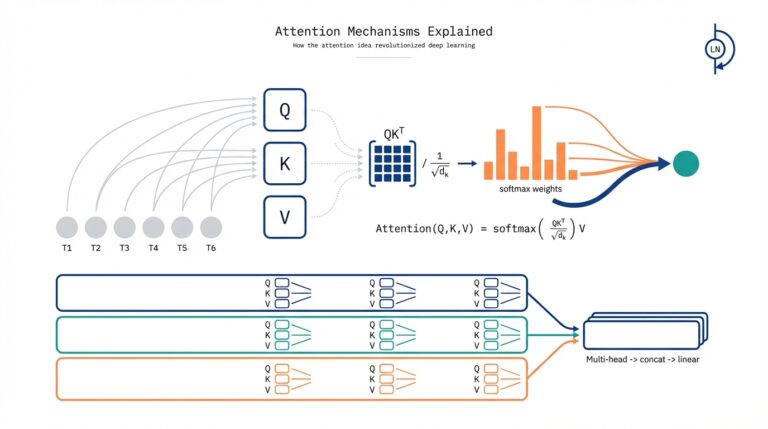
The attention mechanism itself is surprisingly direct: we project inputs into Query (Q), Key (K), and Value (V) vectors and compute weights from the similarity of Q and K; the output is a weighted sum of V. In practice we use the scaled dot-product form: Attention(Q,K,V) = softmax(QK^T / sqrt(d_k)) V, which stabilizes gradients and produces interpretable attention maps that indicate which source tokens influenced each output vector. This formulation turns memory into a matrix operation you can parallelize across tokens and batches, and it gives you immediate diagnostics—inspect the attention matrix to see which tokens the model considered relevant for a given prediction.
In contrast to RNNs and LSTMs, this approach removes recurrence as the main mechanism for carrying context, which yields two engineering benefits: massive parallelism during training and much better handling of long-range dependencies. Because transformers compute attention across all positions in a layer, dependencies spanning hundreds or thousands of tokens can be modeled without vanishing gradients or gated state traversal. The trade-off is computational: naive self-attention scales quadratically with sequence length, so for very long inputs you must choose sparse patterns, chunking, or efficient transformer variants to keep latency and memory within practical bounds.
Operationalizing attention in production requires a few architectural ingredients to make training stable and performant: multi-head attention to let the model attend to multiple relations simultaneously, positional encodings to restore order information, residual connections for gradient flow, and layer normalization for stable optimization. Multi-head attention partitions the projection space so one head can focus on syntax while another captures topical or coreferent relations; positional encodings (sinusoidal or learned) inject a sense of token order that a plain attention matrix lacks. These patterns translate directly into implementation: stack encoder/decoder layers, apply masked attention for autoregressive generation, and use dropout and careful learning-rate schedules (warmup followed by decay) to avoid divergence on large-scale training.
What does this mean in concrete systems you build? For translation and summarization pipelines, replacing recurrent encoders with transformer encoders/decoders typically yields higher BLEU or ROUGE scores while simplifying decoding pipelines. For retrieval-augmented generation and question answering, attention lets you fuse retrieved passage vectors with query representations and condition generation on salient evidence; in practice we fine-tune a transformer on mix-of-domain data and then add sparse attention or memory-compression layers when context grows beyond a few thousand tokens. When latency is critical, you can distill large transformer models into compact student models or adopt efficient attention approximations (Linformer, Performer, or Longformer-style sparse masks) so you maintain high accuracy while meeting production constraints.
Taking this concept further, attention became the foundation for large pretrained models that we fine-tune or adapt for downstream tasks, changing how we engineer transfer learning for language. Because transformer layers produce rich contextual embeddings at every stage, we can reuse pretrained weights, add lightweight adapters, or apply parameter-efficient fine-tuning to get task-specific behavior without retraining the whole model. Building on these mechanics, the next section examines how scaling, pretraining objectives, and deployment strategies shape the design choices you’ll make when integrating transformer-based systems into real-world workflows.
Future Directions: Multimodal and Efficiency
Building on the transformer-era advances we covered earlier, the next phase of practical NLP development converges around multimodal capabilities and model efficiency as co-equal priorities. Multimodal models—systems that jointly process text, images, audio, and structured signals—are becoming a standard requirement for real-world products, but you can only ship them at scale if you prioritize efficiency in training and inference. We’ll examine architectural patterns, tuning tricks, and system-level techniques that let you deliver multimodal functionality without unsustainable compute or latency costs.
At a conceptual level, multimodal means learning representations that let different sensor streams speak the same embedding language. Building on attention, cross-modal attention layers and shared latent spaces let you project image patches, audio frames, and token embeddings into comparable vectors so the model can reason across modalities. Use cases where this matters include image-grounded question answering, video summarization with speech transcripts, and document ingestion pipelines that merge OCR text with layout and visual cues. When should you choose a fused multimodal model versus a pipeline of single-modality models? Choose fusion when tight joint reasoning or end-to-end fine-tuning materially improves downstream metrics; choose modular pipelines when latency, interpretability, or independent model updates are higher priorities.
From an architectural standpoint, two fusion patterns dominate: early fusion (concatenate modality features before deep layers) and late fusion (merge modality-specific encoders via cross-attention or a lightweight combiner). Early fusion gives the model full joint context but increases sequence length and quadratic attention costs; late fusion keeps encoders compact and lets you reuse pretrained uni-modal weights. A practical hybrid is to encode each modality with a specialized encoder (vision transformer for images, waveform encoder for audio, text transformer for tokens) and apply a small number of cross-attention blocks only at deeper layers—this balances cross-modal reasoning with compute economy and speeds retraining when one modality changes.
Efficiency at the model level is no longer optional. Parameter-efficient fine-tuning techniques such as adapters, LoRA (low-rank adaptation), and prompt tuning let you adapt large pretrained backbones to new multimodal tasks with orders-of-magnitude fewer trainable parameters. Quantization and pruning reduce memory footprint and improve inference throughput: 8-bit or 4-bit quantization often preserves accuracy while cutting activation and weight memory dramatically, and structured pruning can lower FLOPs for latency-sensitive deployments. How do you choose between quantization and knowledge distillation? Use quantization when you need immediate memory savings and minimal retraining; use distillation to transfer behavior into a smaller student model when you can afford a training phase that optimizes latency-accuracy tradeoffs.
Operational techniques amplify these model-level gains. Mixed precision (FP16/BF16) halves memory and increases GPU throughput in many workloads; tensor parallelism and model sharding let you spread large multimodal models across devices; and compiler optimizations (XLA, TorchScript, or hardware-specific kernels) squeeze further speedups. For multimodal search and retrieval, augment models with an embedding store and nearest-neighbor index so you can retrieve relevant image or text embeddings instead of fully attending to massive context windows. In one production pattern we use a lightweight vision encoder to produce 512-D vectors, store them in an HNSW index, and only run the heavy cross-attention fusion for the top-k candidates—this reduces average compute per query while preserving end-to-end relevance.
Measuring progress requires explicit efficiency-aware metrics. Don’t only report accuracy; report p95 latency, throughput (queries/sec or tokens/sec), memory footprint, and energy per inference where possible. For multimodal tasks add task-specific signals such as image-text retrieval mAP, captioning CIDEr/ROUGE where appropriate, and human evaluation for grounded generation. Put these metrics in an SLO-driven dashboard so you can trade off a 1–3% accuracy drop for 2x cost savings when that choice makes business sense, and run A/B tests that expose real-user impact rather than relying solely on proxy metrics.
As we continue integrating multimodal reasoning into products, the practical frontier is increasingly about smart allocation of compute: where to spend FLOPs for joint understanding versus where to use fast heuristics and retrieval. In the next section we’ll dig into scaling strategies and safety considerations so you can choose architectures and deployment patterns that meet both user expectations and operational constraints.