Why SQL Still Powers Pipelines
Building on this foundation, we still find SQL at the center of most production data pipelines because it solves problems that transcend tooling trends. SQL’s declarative surface lets you state intent — filter, join, aggregate — and rely on the engine to pick a plan, which accelerates development across ETL/ELT, streaming, and data warehouse stages. For teams, that means fewer brittle scripts and faster handoffs between engineers and analysts. Because the keywords you care about — SQL, data pipelines, ETL/ELT, data warehouse — are front and center in platform roadmaps, choosing SQL aligns your work with the wider ecosystem.
The pragmatic reason SQL survives is execution efficiency: modern engines optimize SQL aggressively. Query optimizers perform predicate pushdown, join reordering, and exploit columnar storage and vectorized execution to make large scans cheap; that translates to lower compute costs and predictable latency in pipelines. Practically, you decide when to push computation down to the warehouse versus pre-computing in a streaming layer based on data freshness and cost; pushdown makes sense when the warehouse can run the same transformation more cheaply and with built-in indexes or clustering. In short, SQL lets us express transformations concisely while the engine handles the heavy lifting.
Operational correctness and governance are another strong argument. Schemas, constraints, ACID transactions, and mature access controls live naturally in SQL-first systems, so you get stronger data quality and easier audits without inventing bespoke controls. How do you maintain correctness across high-volume change data capture (CDC) and time-series ingestion? Use transactional MERGE/upsert patterns and partitioning strategies to ensure idempotency and reproducible backfills, and rely on the warehouse’s lineage hooks to trace upstream sources. Those guarantees reduce incident time and make testing transformations tractable.
The ecosystem around SQL compounds its advantage: orchestration tools, BI platforms, data catalogs, and CI systems all expect SQL artifacts. That means you can version, test, and deploy transformations as SQL files, and integrate them into an orchestration workflow for scheduling, alerting, and incremental runs. For example, we commonly implement CDC-to-warehouse flows with a MERGE pattern: MERGE INTO warehouse.table t USING staging s ON t.id = s.id WHEN MATCHED THEN UPDATE ... WHEN NOT MATCHED THEN INSERT ...; — this single statement captures idempotent behavior, reducing custom script complexity and improving observability.
SQL also bridges batch and streaming semantics in practical ways. Streaming SQL extensions (event-time windows, late-arrival handling, materialized views) let you express continuous computations using familiar constructs like GROUP BY and window functions, so you don’t need a separate DSL for aggregations. For instance, a sliding-window query such as SELECT user_id, COUNT(*) FROM events GROUP BY TUMBLE(event_time, INTERVAL '1' HOUR) maps neatly to both analytical and near-real-time dashboards. That convergence simplifies architecture: you can prototype with SQL, validate results in batch, then incrementally migrate to continuous execution with minimal rewrites.
The implication for engineers is straightforward: invest in good SQL design, testing, and orchestration practices because they buy you velocity, reliability, and cross-functional collaboration. We should treat SQL artifacts as first-class code: lint them, run unit tests against small datasets, and embed them in CI pipelines so deployments are reproducible. As we move to orchestrating complex DAGs and optimizing storage formats, SQL remains the lingua franca that ties ingestion, transformation, and consumption together — which sets up our next discussion on orchestration patterns and how to operationalize SQL-centric pipelines at scale.
Ingestion Patterns: CDC and Connectors
Modern ingestion needs to balance timeliness, correctness, and cost, and the two patterns that deliver that balance most often are CDC (change data capture) and purpose-built connectors. CDC captures granular row-level changes from a source database and streams them as events; connectors are the adapters that normalize and transport those events into your pipeline. By front-loading CDC, connectors, and ingestion into the first 100 words we signal priorities: low-latency updates, transactional fidelity, and predictable upserts into your warehouse. We’ll assume you already value SQL-based MERGE/upsert patterns from the previous section and show how CDC and connectors feed them reliably.
Start with the trade-offs: use log-based CDC when you need near-real-time state replication, auditability, and minimal load on the source database; use batch connectors when throughput is high, freshness windows are loose, and cost matters more than sub-second latency. Log-based CDC (reading the database transaction log) preserves ordering and transactional boundaries, which simplifies idempotent application of changes downstream. In contrast, file or API-based connectors are simpler to deploy and often cheaper for large-volume bulk loads but require additional logic for deduplication and change ordering.
A pragmatic architecture looks like this: CDC producer → connector (transform/tombstone handling) → streaming transport (Kafka, Pub/Sub) → staging table in the warehouse → transactional MERGE into the canonical table. Use a small, durable staging schema to capture _op_type, _lsn/_position, _commit_ts, and raw payload; those metadata fields let you implement deterministic MERGE logic. For example, you can upsert with a MERGE statement that respects delete tombstones and commit timestamps to resolve concurrency:
MERGE INTO canonical.orders AS t
USING staging.orders_s AS s
ON t.order_id = s.order_id
WHEN MATCHED AND s._op = 'DELETE' THEN DELETE
WHEN MATCHED AND s._commit_ts > t._commit_ts THEN
  UPDATE SET status = s.status, qty = s.qty, _commit_ts = s._commit_ts
WHEN NOT MATCHED THEN
  INSERT (order_id, status, qty, _commit_ts) VALUES (s.order_id, s.status, s.qty, s._commit_ts);
How do you ensure exactly-once semantics in a CDC-to-warehouse flow? You rarely get true exactly-once without end-to-end transactional support, so optimize for idempotency and deterministic conflict resolution. Persist source positions (LSNs) with each batch commit, use deduplication keys that include source position or a natural unique key, and design your MERGE logic to prefer the highest commit timestamp. Handle tombstones explicitly so deletes don’t get replayed as inserts; for schema evolution, use a schema registry or the connector’s schema support to emit explicit add/drop events and avoid silent field loss.
Operational signals matter as much as correctness. Monitor connector lag, record backpressure from streaming layers, and set retention/compaction policies to avoid unbounded storage growth. Micro-batch windows (1–30 seconds) are a practical compromise between latency and write amplification for many warehouses; smaller windows increase load and cost but reduce end-to-end latency. We also recommend integrating connector health into your orchestration—failures in the connector should trigger downstream DAG pauses and alerting so you don’t absorb corrupted or partial change batches.
In practice, choose CDC and connector strategies that align with downstream SQL patterns and your SLAs: prefer log-based CDC for near-real-time analytics and fraud detection, use scheduled connectors for nightly backfills and large table snapshots, and standardize on merge-based, idempotent SQL transformations to absorb variability. By treating connectors as first-class pipeline components and encoding deterministic merge rules in SQL, you keep the guarantees and observability you need while leveraging the performance and governance benefits we described earlier. This sets up the orchestration decisions and incremental modeling we’ll cover next.
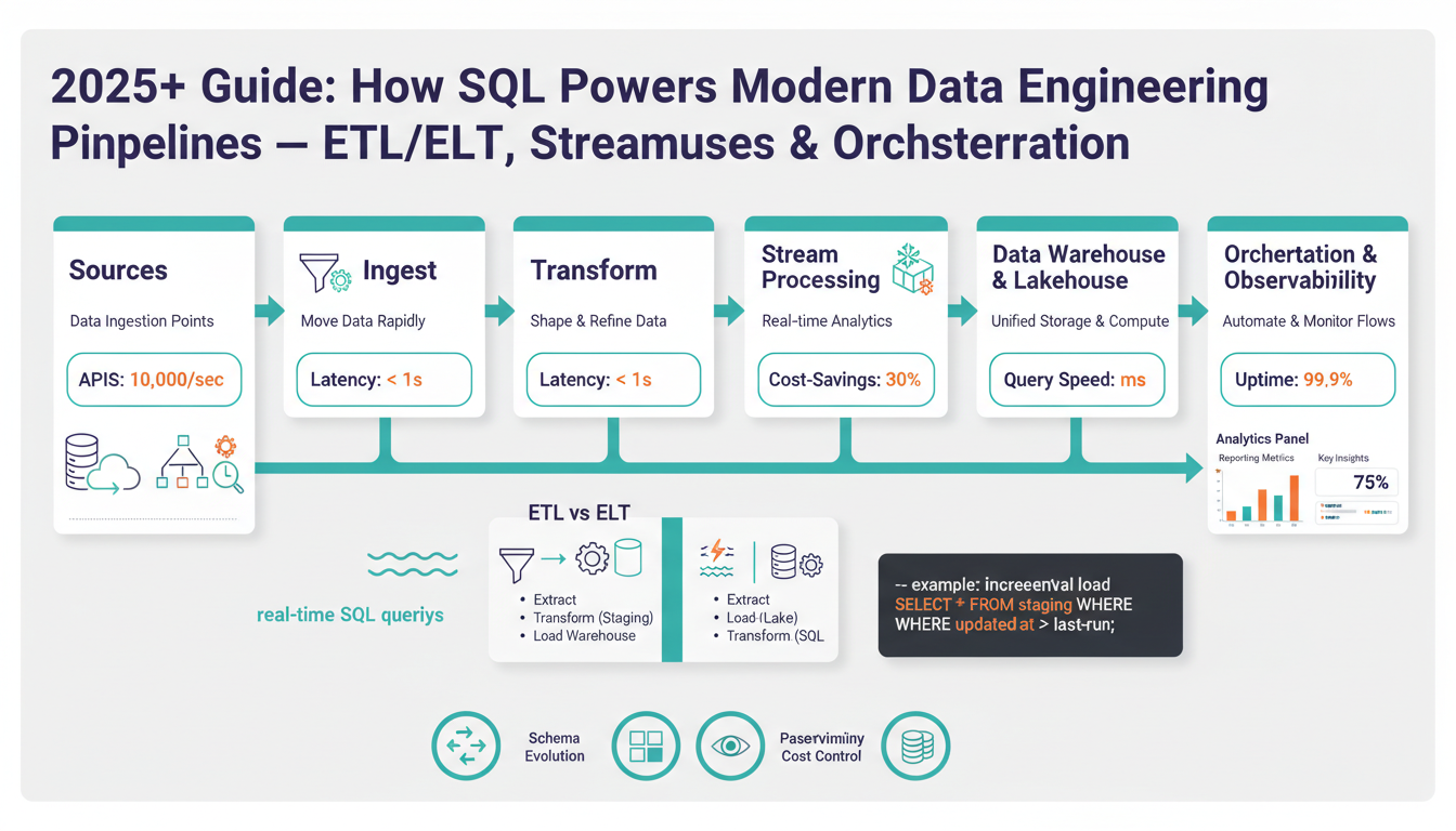
Batch ETL Versus ELT Transformations
Choosing where to run transformations is one of the most consequential architecture decisions you make for a data pipeline: do you transform upstream in batch ETL or load raw data and transform inside the warehouse with ELT? This question shapes cost, latency, governance, and developer velocity from day one. Building on our earlier points about SQL’s centrality and MERGE/upsert patterns, we should treat this as a trade-off between pre-computation and pushdown: batch ETL pre-computes outside the data warehouse, while ELT relies on SQL and the warehouse’s optimizer to do the heavy lifting after load.
Batch ETL means you extract, transform, then load a curated, consumable dataset into downstream storage or a warehouse. You typically run transformations in Spark, Flink, or other batch engines where you can implement complex logic, custom libraries, or heavy joins without incurring expensive warehouse compute. This approach is appropriate when regulatory requirements demand transformed, masked, or aggregated records before landing, or when source systems cannot tolerate extraction patterns that preserve ordering and idempotency. Operationally, batch ETL isolates transformation failures from the warehouse, simplifies lineage for upstream teams, and often reduces warehouse storage but can increase pipeline latency and operational surface area.
ELT flips that sequence: load raw or minimally cleaned data into staging and perform transformations with SQL inside the warehouse. ELT leverages the warehouse’s predicate pushdown, columnar storage, clustering, and query optimizer so your transformations become maintainable SQL artifacts that we can version, test, and orchestrate. This model accelerates iteration—analysts and engineers can prototype with CREATE TABLE AS SELECT or MERGE statements and rely on the engine to scale execution. ELT reduces data movement, centralizes governance, and aligns with the broader ecosystem that expects SQL artifacts. The trade-off is that complex, expensive operations (wide shuffles, heavy machine learning featurization, or high-cardinality joins) can become costly if run entirely in-database.
How do you decide between them? Base the choice on three practical criteria: cost curve, transformation complexity, and SLA for freshness. If compute in your warehouse is expensive per TB scanned and you have repeated heavy aggregates, pre-aggregating in a batch ETL job can be cheaper. If you need sub-hour freshness, flexible schema evolution, and tight collaboration with analysts, ELT’s agility usually wins. For mixed constraints, adopt a hybrid rule: precompute extremely expensive or non-SQL-friendly steps upstream, then load and finalize business logic using SQL models. This decision framework keeps the data pipeline aligned with both cost targets and product SLAs.
In practice, most production systems use a hybrid pattern rather than a pure binary choice. We often push deterministic deduplication, primary-key reconciliation, or complex feature engineering into a scheduled batch job, then use incremental ELT models for denormalization, lookups, and applied business rules. For example, pre-aggregating per-user session metrics in Spark reduces cardinality, and a downstream MERGE into the canonical table applies business constraints and lineage metadata. Make transformations idempotent, persist source positions for CDC-based flows, and instrument both sides with the same data quality checks so comparisons between batch and ELT results are straightforward during migrations.
Design your transformations for testability and observability regardless of where they run. Treat SQL models as first-class code, write unit tests against small datasets, and enforce schema contracts at the staging boundary. Monitor cost and query plans for ELT models and maintain a catalog of which transformations are precomputed vs pushed down so operators can reason about latency and failure modes. Taking this concept further, the orchestration layer should be able to run hybrid DAGs—pause downstream consumers when upstream ETL fails, trigger incremental ELT runs after a CDC micro-batch, and surface lineage so you can trace a row from source to dashboard. That operational clarity is what lets us scale SQL-centric pipelines while keeping cost and correctness under control.
Streaming SQL: Stateful Processing Examples
Building on the patterns we discussed earlier, real-time pipelines often require stateful computations that evolve as events arrive — not just stateless filters or simple enrichments. Stateful processing means you keep and mutate per-key context (counters, windows, last-seen timestamps, or complex session state) across event streams so downstream SQL can answer questions like session length, running conversion rates, or time-windowed aggregates. If you design these flows with SQL-first tooling, you get the declarative clarity of GROUP BY and window functions while still encoding the operational rules for correctness and recovery.
At a technical level, stateful streaming keeps key-partitioned state and uses event-time semantics to make results deterministic. Event-time processing uses timestamps embedded in events rather than arrival time; watermarks (a progress signal indicating how far event-time has advanced) let engines close windows and evict state. Define a watermark on first use: a watermark is an estimate of the maximum event-time seen so far, used to decide when to emit final results for a window. Practically, you choose processing-time only for best-effort metrics and event-time plus watermarks for correctness-sensitive use cases like billing, analytics, or fraud detection.
Common SQL patterns implement windows and stateful aggregates without custom code. Tumbling windows (fixed, non-overlapping), hopping/sliding windows (regularly overlapping), and session windows (gap-based grouping) cover most needs and map directly to SQL extensions: for example, SELECT user_id, COUNT(*) FROM events GROUP BY TUMBLE(event_time, INTERVAL ‘1’ HOUR). You can express sessionization with SESSION(event_time, INTERVAL ‘30’ MINUTE) to group user activity into sessions. These constructs let you move from batch prototypes to continuous queries with minimal rewrites, keeping the same GROUP BY and window logic across modes.
Late arrivals and corrections are the hardest part of stateful pipelines; we handle them by combining watermarks, retractions, and materialized-change outputs. Many engines emit changelog rows (retract/insert pairs) or support upsert-materialized views so you can persist incremental deltas to a durable table. For warehouse-backed flows, implement a deterministic MERGE that prefers the highest event_time or commit_ts and treats tombstones explicitly; for example, MERGE INTO sessions USING staging ON … WHEN MATCHED AND s._op=’DELETE’ THEN DELETE WHEN MATCHED THEN UPDATE … WHEN NOT MATCHED THEN INSERT …; this pattern keeps state convergent after replays or late events.
To make stateful SQL practical at scale, you need explicit state management choices: tombstone handling for deletes, TTLs (time-to-live) to bound state size, and checkpointing to enable fast recovery. For instance, implement a session table keyed by user_id with columns (session_id, last_event_ts, event_count) and update it incrementally from streaming aggregates; compact old sessions with TTL and emit final session summaries to an analytical table. Also partition keys consistently (hash by user_id) to avoid hotspots and tune state backend settings (snapshot frequency, incremental checkpoints) so checkpoint durations don’t become your operational bottleneck.
How do you validate stateful logic before it runs in production? Unit-test streaming SQL by running small deterministic event traces through the same windowing and watermark rules you’ll use in production, then assert the expected changelog output. Maintain end-to-end replay tests that reingest historical data into your micro-batch or continuous engine to exercise MERGE-idempotency and late-arrival reconciliation. Monitor state growth, checkpoint latency, watermark lag, and per-partition processing time in production; those metrics reveal whether state is compounding or if backpressure will eventually stall the pipeline.
Taking these examples further, treat your stateful SQL queries as first-class artifacts in the pipeline: version them, run regression tests, and let the orchestration layer coordinate backfills and streaming deployments. By combining event-time windows, watermarks, materialized views (or changelog tables), and deterministic MERGE/upsert patterns, you preserve correctness while delivering low-latency insights. Next, we’ll look at how orchestration and incremental modeling tie these continuous computations into reliable production workflows.
Modern Warehouses and Storage Formats
Building on this foundation, modern data warehouse design is as much about where you store bytes as it is about how you express transformations in SQL. You should treat the choice of storage formats and table abstractions as a first-class architecture decision because they determine query latency, cost per terabyte scanned, and the operational complexity of CDC and streaming flows. When we pick a storage layer, we’re choosing the primitive that enables predicate pushdown, columnar scans, snapshot isolation, and efficient incremental MERGE patterns — all features that let SQL remain the lingua franca across ingestion, transformation, and consumption. This matters for pipelines that need sub-minute freshness and for analytical workloads that scan petabytes of historical data alike.
Why choose a managed cloud warehouse versus an open table format on object storage? That question should drive your initial evaluation. Managed warehouses (Snowflake, BigQuery, cloud-native warehousing) give you turnkey clustering, storage/compute separation, and aggressive optimization out of the box, which reduces operational burden. Open table formats (Delta Lake, Apache Iceberg, Apache Hudi) on object storage give you portability, cheaper archival, and explicit control over compaction, snapshots, and metadata — which matters if you need cross-engine reads or want to avoid vendor lock-in. We recommend evaluating based on three things: your query SLA and concurrency requirements, your tolerance for operational overhead (compaction, metadata service), and whether you need multi-engine access to the same underlying data.
At the file level, columnar storage formats like Parquet and ORC remain the workhorses for analytical performance. Columnar layouts enable column pruning and vectorized execution, which dramatically reduce I/O for wide tables; predicate pushdown lets engines skip entire row groups or files when predicates are selective. In practice, tune partitioning and file sizes: avoid overly granular date partitions that produce many small files, and target larger file sizes (hundreds of megabytes to ~1GB per file for high-throughput workloads) to maximize read efficiency. Use hash or bucket partitioning for high-cardinality keys when you need efficient joins or shuffles, and apply sort/clustering keys for frequently filtered columns so you get better data locality and fewer scanned pages.
Table formats add the transactional and schema guarantees you need for production pipelines. Delta, Iceberg, and Hudi provide ACID semantics, snapshot isolation, time travel, and explicit schema-evolution primitives so you can apply deterministic MERGE/upsert patterns from CDC and streaming sources without corrupting the table. These formats also expose metadata (manifests, snapshot catalogs) that query engines use for fast partition pruning and incremental reads; that’s how you can run an efficient MERGE that only touches touched partitions instead of scanning the whole table. Operationally, plan for compaction and metadata maintenance: periodic compaction reduces small-file overhead and snapshot pruning keeps metadata operations fast as your table ages.
Operational patterns matter more than theoretical advantages. A robust pipeline stages raw events in an object store using append-only Parquet files, writes micro-batches indexed by commit_ts, runs a compact/optimize job to rewrite files into larger columnar segments, and then performs transactional MERGE into the canonical table format. Monitor small-file ratios, read amplification, and metadata operation latency; automate compaction when the small-file percentage crosses a threshold and expose table-level TTL or retention policies to bound storage. For cost control, pre-aggregate extremely expensive joins upstream when those operations would repeatedly scan large historical partitions, and leave business logic, joins, and denormalization to SQL models inside the warehouse or table-engine where predicate pushdown and clustering reduce repeated work.
These storage and table format choices have direct governance and testing implications: choose formats that integrate with your catalog, lineage tooling, and access controls so you can audit transformations and trace rows end-to-end. We should version table schemas, include snapshot-based regression tests for MERGE logic, and surface compaction and checkpoint health to the orchestration layer so backfills and streaming deployments behave predictably. Taking this approach lets SQL remain the single language for expressing transformations while you rely on modern storage formats and warehouse features to deliver performance, correctness, and operational scalability — which leads naturally into how we orchestrate incremental models and recovery in production.
Orchestration Testing Deployment Best Practices
Building on this foundation, treat SQL, orchestration, testing, and deployment as a single lifecycle you can automate and observe. The fastest way to break a production pipeline is to treat transformations as one-off queries and schedule them without CI. Instead, version SQL artifacts, run linting and unit tests, and gate deployments through an automated pipeline so changes to models or MERGE logic carry the same quality gates as application code. This approach reduces regressions and makes pipeline behavior reproducible across environments.
Start with test tiers that match how you build models: unit tests for SQL logic, integration tests for upstream connectors and staging tables, and end-to-end tests for DAG-level correctness. How do you validate that a MERGE is idempotent, or that a stateful sliding-window query tolerates late arrivals? Write deterministic small-trace tests that assert expected changelog outputs, include schema-contract checks that fail fast on type changes, and add regression tests that compare current output to a canonical snapshot. Use generated fixtures (a few dozen rows) to exercise boundary cases—null-heavy rows, duplicate keys, tombstones—and run them locally and in CI with the same SQL engine used in production.
Integration testing needs environment parity and replayability so you can exercise CDC and streaming semantics. Create a staging environment that mirrors production table formats and snapshot semantics, then replay recorded CDC batches or event traces into the pipeline to validate ordering, watermark behavior, and MERGE conflict resolution. Persist source positions (LSNs or offsets) in test runs so you can assert idempotency by replaying the same trace twice; your assertions should check both row-level checksums and business invariants (no lost deletes, monotonic timestamps, unique keys preserved). Automate schema-evolution smoke tests by applying additive and non-destructive changes and running downstream queries that surface silent field loss.
For deployment, build a CI/CD flow that enforces immutability and safe promotion: lint and unit tests on pull request, integration and snapshot regression tests on merge, deploy to staging for a smoke window, and promote to production only after health checks pass. Treat DDL and DML separately: use a migration table or a schema-change job to apply DDL with explicit review, and deploy SQL models by promoting versioned artifacts to the orchestrator. Use feature flags or a toggle table for risky transformations so you can flip behavior without code changes. Keep deployments atomic where possible and ensure your orchestrator supports transactional run contexts or compensating actions when partial runs fail.
Tune the orchestrator for operational resilience: design idempotent tasks, prefer task-level checkpointing over global state, and expose backfill controls so operators can restart ranges without manual patching. Integrate sensors for connector lag, streaming watermark delays, and small-file ratios so DAGs pause or degrade gracefully when upstream health falters. Implement canary runs for expensive or high-impact models—run new logic on a sampled partition or a slice of customer data, compare metrics, then promote. Parameterize runs (date, watermark, batch-id) so backfills and replays are deterministic and fully auditable.
Observability and rollback matter as much as tests and deployment gates. Surface lineage and row-level provenance for high-risk tables, emit business-level SLAs from jobs (rows_processed, commit_ts, lag_ms), and wire automated alerts to fail fast. When a deployment introduces a regression, prefer automated rollback and a gated backfill that replays only the affected partitions using idempotent MERGE logic. Taking these practices together makes orchestration, testing, and deployment a continuous loop: we test against production-like traces, we deploy through guarded promotions, and we monitor and rollback confidently so pipelines recover predictably. Building on this, the next section will show how incremental modeling and recovery patterns integrate with orchestrated deployments to minimize downtime and reprocessing cost.