What is Gradient Descent? A Conceptual Overview
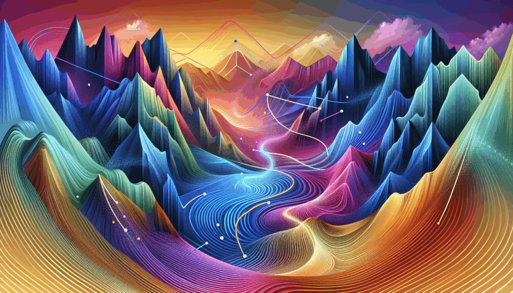
Imagine you are standing on a foggy mountain, trying to find your way down to the lowest point. You don’t have a map—all you can do is feel the slope beneath your feet, then take a cautious step in the direction that seems to go downhill. This real-world intuition beautifully mirrors the mathematical method known as gradient descent.
At its core, gradient descent is an iterative optimization algorithm used to minimize a function—most commonly a cost or error function found in machine learning and data science applications. It systematically adjusts a model’s parameters to reduce errors and improve predictions. The process may sound simple, but its impact is profound, powering everything from image recognition to natural language processing.
Conceptually, what is happening? Every machine learning model aims to make predictions as accurately as possible. This accuracy (or inaccuracy) is quantified using a loss function, which measures the difference between predicted values and the real, known values. The lower this value, the better the model. However, finding the right set of parameters that yield the lowest loss is rarely straightforward—it’s often like searching for the deepest point in a vast, multi-dimensional landscape filled with hills and valleys (local minima and maxima).
The “gradient” in gradient descent refers to the vector of partial derivatives of the loss function with respect to the model’s parameters. This gradient essentially points in the direction of the steepest ascent. To minimize the loss, we want to go in the opposite direction—downhill. Google’s Machine Learning Crash Course provides a visual explanation of how gradients work in optimization.
Iterative Steps of Gradient Descent:
- Start with an initial guess for the parameters (weights).
- Calculate the gradient (slope) of the loss function at that set of parameters.
- Take a step in the opposite direction of the gradient—this “step” is scaled by a parameter called the learning rate.
- Update the parameters with the new values and repeat the process.
- Continue until the change in loss function or the parameter values is minimal, indicating convergence.
Consider a practical example using linear regression: Suppose you’re trying to fit a straight line to a set of data points. The objective is to find the slope and intercept that minimize the sum of squared differences between the predicted and actual values. Gradient descent allows you to systematically “slide” these parameters to their optimal settings, even with thousands of features or data points, making it a cornerstone of modern machine learning and statistical modeling (Carnegie Mellon Statistics Lecture).
While there are numerous variants—such as stochastic gradient descent and mini-batch gradient descent—the central idea remains unchanged: gradually hone parameter values to minimize error. This journey from the randomness (chaos) of initial guesses to the harmony (convergence) of minimum error is what makes gradient descent both mathematically elegant and practically powerful.
The Mathematical Foundation: Gradients and Loss Functions
At the heart of gradient descent lies a powerful interplay between gradients and loss functions. These fundamental mathematical concepts work together to guide an algorithm from a wild landscape of random parameters toward a well-tuned solution. To truly understand how gradient descent operates, it’s important to explore both the theoretical underpinnings and the real-world mechanics of these elements.
Gradients: Imagine standing on a mountain surrounded by fog, wanting to reach the lowest point in the valley. You can’t see far, but you can sense which direction the ground slopes downward beneath your feet. In mathematical terms, this slope is represented by the gradient. The gradient is a vector that points in the direction of the steepest increase of a function. In the context of optimization, however, we’re interested in descending—so we move in the opposite direction of the gradient.
Mathematically, if you have a function that takes several inputs—like the weights in a neural network—the gradient at any point is a vector of partial derivatives with respect to those inputs. For example, if your function is f(x, y), the gradient is written as:
∇f(x, y) = [∂f/∂x, ∂f/∂y]This tells you how rapidly the function increases if you nudge x or y just a little, and in which directions.
Loss Functions: Quantifying the Chaos
Before any optimization can happen, you need a way to measure how well your model is performing—or, more specifically, how far it is from the ideal. This measurement is provided by the loss function. Think of a loss function like a scorekeeper in a game: it assigns a numerical value to the difference between your model’s predicted output and the actual, desired result. In machine learning, common loss functions include mean squared error for regression and cross-entropy for classification.
- Example 1: If you’re predicting house prices, the loss might be the average squared difference between predicted and actual prices.
- Example 2: For classifying images, the loss is higher when the model is less confident (and more wrong) about its classifications.
A well-chosen loss function shapes the “terrain” that gradient descent traverses. A good loss function not only informs the model how wrong it is, but also ensures the gradient points toward better solutions—think of it as part map, part compass.
Bringing Gradients and Loss Together: The Cycle
Here’s how these ideas interlock seamlessly in a step-by-step process:
- Start with a random set of parameters for your model.
- Measure the loss by plugging these parameters into your loss function.
- Calculate the gradient of the loss function with respect to each parameter.
- Update the parameters in the direction opposite to the gradient—this should reduce the loss.
- Repeat the process until visiting new parameter values yields negligible improvements.
This process transforms chaos—the initial random guesses—into convergence on an optimal (or at least much-improved) solution. If you’d like to see a visual step-through, 3Blue1Brown’s visual explanation of gradient descent is an industry favorite.
In summary, the dynamic between gradients and loss functions forms the mathematical engine of learning for algorithms, allowing them to iteratively improve and learn from their mistakes—one calculated step at a time.
Types of Gradient Descent: Batch, Stochastic, and Mini-Batch
When diving deeper into gradient descent, it’s crucial to understand that there isn’t just one unified approach. In fact, the method varies based on how much data is used during the update of parameters. Let’s explore the most common techniques—Batch, Stochastic, and Mini-Batch Gradient Descent—each with its unique strengths, weaknesses, and best-use scenarios.
Batch Gradient Descent
Batch Gradient Descent computes the gradient of the cost function with respect to the parameters for the entire training dataset. In other words, it uses all available data before updating model weights, resulting in highly accurate and stable updates. The process looks like this:
- Step 1: Compute the gradient of the cost function by averaging across all training examples.
- Step 2: Update the parameters using these gradients.
- Step 3: Repeat until convergence is achieved.
Example: If you have a dataset with 10,000 samples, each iteration (or epoch) processes all 10,000 before making a single update to the model.
Advantages: The updates are less noisy, making it easier to reach global minima (Google Developer’s Guide). This method is best for smaller datasets where computational resources are not a constraint.
Drawbacks: For large datasets, computations are slow, and memory requirements can be a bottleneck. If your data can’t fit into memory, batch gradient descent becomes infeasible.
Stochastic Gradient Descent (SGD)
Stochastic Gradient Descent dramatically changes the approach by updating parameters for each training example, one at a time.
- Step 1: Randomly shuffle the dataset.
- Step 2: For each training example, calculate the gradient and update the parameters immediately.
- Step 3: Repeat the process for several passes through the dataset (epochs).
Example: In a dataset of 10,000 samples, each parameter update is made after processing just a single example, leading to 10,000 updates per epoch.
Advantages: Allows the algorithm to start learning before having the whole dataset processed and can escape shallow local minima due to its noisier updates. This property is extremely useful in online learning scenarios and for huge datasets (University of Toronto Lecture Slides).
Drawbacks: The noisiness of updates can make convergence slower and less stable, often requiring advanced optimization techniques—like learning rate schedules or momentum—to tame the oscillations.
Mini-Batch Gradient Descent
Mini-Batch Gradient Descent is a hybrid approach that strikes a balance between the stability of batch processing and the efficiency of stochastic updates. Instead of using all examples or just one, data is split into small batches (e.g., 32, 64, 128 samples), and parameter updates are performed on each batch.
- Step 1: Divide the dataset into small batches.
- Step 2: For each batch, calculate the gradient and update the parameters.
- Step 3: Repeat for all batches in each epoch, until the algorithm converges.
Example: With a dataset of 10,000 samples and a batch size of 100, there will be 100 updates per epoch—each after processing a mini-batch.
Advantages: Combines faster computation with improved convergence properties. Mini-batch updates efficiently utilize modern hardware (like GPUs), making it central to deep learning frameworks (DeepLearning.AI Glossary).
Drawbacks: Choosing the right batch size requires experimentation. Too small, and learning is as noisy as SGD; too large, and it starts behaving like batch gradient descent with the accompanying resource strain.
Each type of gradient descent offers a different trade-off between speed, accuracy, resource use, and stability. The choice fundamentally shapes model training dynamics, making it essential knowledge for understanding and deploying effective machine learning algorithms. For more in-depth mathematical nuances, see Cornell University’s Lecture Note on Gradient Descent.
Visualizing the Descent: Intuition and Graphical Insights
Imagine standing at the top of a foggy mountain with the goal of finding the lowest valley. Every step you take is a careful decision, made using the slope beneath your feet. In machine learning, this journey is called gradient descent. But what does this descent really look like, and how can we intuitively understand and visualize what is happening?
The process of gradient descent can initially feel like stepping into mathematical chaos – full of jagged terrain, shifting directions, and uncertain progress. However, with the help of graphical insights and intuitive examples, we can bring structure and clarity to this journey.
The 3D Landscape: Visualizing the Loss Function
At the heart of gradient descent is the loss function, which can be thought of as a 3D landscape with hills and valleys. The height at each point on the landscape corresponds to the error (or loss) for a particular set of model parameters. To understand this, picture a trampoline stretched into unusual shapes—the lowest dip represents the parameters that minimize the loss.
When you perform gradient descent, you start at a random spot on this landscape and take iterative steps in the direction of the steepest descent. With each step, you consult the local slope—this is the “gradient.” The point-by-point process is beautifully illustrated in this interactive visualization by 3Blue1Brown, an acclaimed mathematics explainer.
Step-by-Step Descent: Learning Through Visualization
To break it down:
- Pick a Starting Point: Imagine a small ball dropped somewhere on the surface. This represents your initial guess for the model’s parameters.
- Calculate the Slope (Gradient): At its current location, the ball “feels” the steepness and direction of the slope beneath it, just as gradient descent computes the partial derivatives of the loss with respect to each parameter.
- Take a Step: Guided by the gradient, the ball moves a small distance downhill. The size of this step is controlled by the learning rate—a crucial factor that determines how fast or slow you move. For a detailed breakdown, check out Stanford University’s CS231n notes on optimization.
- Repeat: This process is repeated, with each movement recalculating the local gradient and nudging the ball ever closer to the bottom of the valley—ideally, the global minimum.
The Role of the Learning Rate: Finding the Right Pace
The learning rate is a hyperparameter that dictates the step size. Too large, and you risk overshooting the valley or bouncing chaotically; too small, and you creep slowly, perhaps never reaching the valley in reasonable time. This is often depicted in visual animations, where you can literally see the difference: large steps cause wild oscillations, while small steps make slow, smooth progress. Harvard’s calculus tutorial provides an excellent example of these dynamics in action.
Contours: 2D Views for Clearer Intuition
Another common and powerful visualization is the contour plot—a 2D top-down view of the loss surface. Here, concentric closed loops represent lines of equal error. Following the path of gradient descent on a contour map helps us appreciate the challenge of navigating curved and elongated valleys. This is essential for understanding how gradient descent tackles real optimization problems, particularly when dealing with multiple features and parameters.
Animation: Watching Convergence Happen
Modern tools and libraries let us animate the path of gradient descent, stepping frame by frame across the loss surface. These animations reveal not only how the algorithm moves but also how it sometimes gets stuck in local minima or plateaus. Such visualizations are invaluable for developing intuition and can be explored interactively in many Jupyter Notebook environments, as demonstrated by experts like Sebastian Raschka, a leading machine learning teacher.
By engaging with these visualizations and building a mental picture, we can transform the seeming chaos of optimization into a process that is not only rigorous and logical but also deeply intuitive.
Common Challenges: Local Minima, Saddle Points, and Learning Rates
Local Minima
One of the main challenges faced when applying gradient descent in machine learning and optimization is navigating the complex terrain of the cost function, especially when it comes to local minima. A local minimum is a point in the parameter space where the function value is lower than all nearby points, but not necessarily the lowest overall. In high-dimensional problems, such as those encountered in deep learning, the cost surface can contain numerous dips and valleys, making it easy for gradient descent to settle in one of these traps rather than the true global minimum.
For example, imagine hiking in a landscape filled with hills and valleys. If you always take the steepest downward path, you might end up in a shallow depression while a deeper valley lies nearby, but out of reach using your current path. This is analogous to how basic gradient descent can get stuck in local minima.
Researchers have devised several strategies to mitigate this, such as:
- Multiple Random Initializations: Start gradient descent from different points in the parameter space to increase chances of finding the global minimum.
- Adding Noise: Introducing random noise to the gradients can help escape shallow local minima by making the optimization process less deterministic.
- Advanced Algorithms: Methods like Stochastic Gradient Descent (SGD) and its variants use batch sampling to provide inherent randomness, aiding in overcoming poor local optima.
Saddle Points
Saddle points can be even trickier than local minima. These are points where the gradient is zero, but the point is neither a minimum nor a maximum. Instead, the cost function curves up in one direction and down in another—imagine the top of a mountain ridge or a saddle on a horse. In high-dimensional spaces, saddle points are far more common than local minima, and gradient descent algorithms can spend a lot of time lingering near these flat regions.
The problem with saddle points is that traditional gradient descent sees no clear path downward, leading to slow progress or stagnation. Some practical remedies include:
- Momentum-Based Methods: Techniques like momentum accumulate past gradients to build velocity and help carry the iterate through flat or problematic regions.
- Adaptive Learning Rates: Algorithms such as Adam or RMSProp adjust learning rates based on past gradients, which can help navigate the flatness of saddle points more efficiently.
- Second Order Methods: These involve curvature information (like the Hessian matrix) to distinguish between minima and saddle points, though they can be computationally expensive.
Learning Rates
The learning rate is arguably the most vital hyperparameter in gradient descent. It dictates the size of the steps taken towards the minimum. Setting this value too high can cause the process to diverge or oscillate wildly, missing the minimum altogether. Conversely, a learning rate that’s too small slows down convergence dramatically, making optimization inefficient and potentially leading to premature stopping.
Choosing the right learning rate requires careful tuning and often, experimentation. Techniques to address learning rate challenges include:
- Learning Rate Scheduling: Start with a higher learning rate and decrease it over time as convergence progresses. This approach is used in deep neural networks to allow quick exploration early on, transitioning to fine-tuning later.
- Adaptive Approaches: As mentioned before, optimizers like Adam and Adagrad automatically adjust the learning rate for each parameter, offering finer control and better performance across different landscapes.
- Manual Tuning: Visualize the loss curve or use cross-validation to experiment with different rates until steady and rapid convergence is observed.
For a hands-on explanation, check out the MIT OpenCourseWare tutorial on gradient descent algorithms, which delves into the practical side of learning rate selection.
Mastering these three elements—local minima, saddle points, and learning rates—provides the foundation for efficiently steering gradient descent from mathematical chaos toward convergence. By understanding and addressing these challenges, practitioners and researchers can improve their models and make optimization a more predictable journey.
Techniques for Faster and More Stable Convergence
One of the core challenges in implementing gradient descent effectively is ensuring that the algorithm converges quickly and stably to an optimal solution. Over the years, a range of techniques and best practices have been developed to address these challenges. Below, we explore some of the most impactful approaches, supported by examples and insights from leading research.
Choosing the Right Learning Rate
The learning rate determines how big each update step is during training. If it’s too high, the algorithm may overshoot minima or even diverge; if it’s too low, convergence becomes painfully slow. A sound method for selecting a learning rate is to start small (e.g., 0.001) and use techniques like learning rate schedules, where the learning rate is gradually decreased as training progresses.
For example, you might use an exponential decay schedule, lowering the rate every few epochs to encourage finer and more stable optimization as the solution approaches the minimum. Experimentation is key—try plotting loss curves with different rates to visually assess stability and speed.
Momentum and Adaptive Methods
Momentum is a technique inspired by physics that helps accelerate gradient descent, especially in the face of noisy or inconsistent gradient directions. By considering the past gradients exponentially, momentum helps the optimizer “push through” flat or oscillating regions of the loss landscape.
- Momentum Example: At each step, maintain a running average of past gradients and add a fraction of this average to the current update.
- Nesterov Accelerated Gradient: An improved version that peeks ahead before computing the update, further stabilizing the path to convergence.
Adaptive methods like RMSProp and Adam dynamically adjust the learning rate for each parameter based on recent gradient information, enabling faster convergence on complex problems. These optimizers have become staples in deep learning due to their ability to handle sparse gradients and varying curvature across the loss surface.
Batch Normalization
Another significant advancement is batch normalization, which normalizes the input of each layer to stabilize the learning process. By reducing the “internal covariate shift,” batch normalization allows larger learning rates and speeds up training, while also providing a regularization effect that can reduce overfitting.
To use batch normalization effectively, add a batch normalization layer after each dense or convolutional layer in your network. During training, the layer normalizes activations to zero mean and unit variance, then scales and shifts them based on learned parameters.
Using Mini-Batches and Stochastic Approaches
Full-batch gradient descent can be computationally expensive and slow, especially on large datasets. Mini-batch and stochastic gradient descent (SGD) offer a solution by updating parameters using only a subset of data at each step.
- Randomly shuffle the dataset at the start of each epoch.
- Divide the data into mini-batches (e.g., 32 or 128 examples).
- Update the model parameters for each mini-batch using the averaged gradients.
This not only speeds up training but adds a beneficial noise to the updates, which can help escape local minima and lead to better overall convergence. For more on the advantages and practices of batch sizing, see Stanford’s CS231n lecture notes.
Early Stopping and Checkpointing
To prevent overfitting while maintaining fast convergence, employ early stopping. This technique monitors a validation metric and halts training once progress stalls, averting wasted computation and potential overfitting. Conservative checkpointing—saving model weights at regular intervals—ensures that you can resume from the latest best state in case of interruptions or diminishing returns.
Summary
Mastering these techniques will help you achieve faster and more stable convergence when training neural networks or any models involving gradient descent. Remember, finding the right combination of strategies often comes down to experimentation and close monitoring of training metrics. As you explore each approach, consult both textbook resources and recent research to evaluate their impact on your specific task and dataset.