XOR problem overview
Exclusive OR (XOR) returns 1 when exactly one of two binary inputs is 1 and 0 otherwise. A compact truth table:
0 XOR 0 = 0
0 XOR 1 = 1
1 XOR 0 = 1
1 XOR 1 = 0
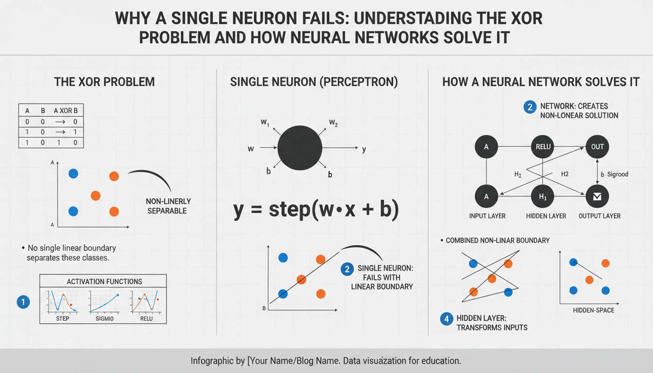
Geometrically, plot the input pairs (0,0), (0,1), (1,0), (1,1) in 2D: the positive outputs lie on opposite corners ((0,1) and (1,0)). A single artificial neuron computes a linear function followed by a threshold (or a sigmoid), so its decision boundary is a straight line. No straight line can separate those diagonal positives from the diagonal negatives, so a single linear unit cannot represent XOR — XOR is not linearly separable.
Solving XOR requires nonlinearity or additional layers. A minimal feedforward network uses one hidden layer with two nonlinear units to transform the input space (for example, implementing intermediate AND/OR-like features) and a final unit to combine them. That hidden transformation creates a piecewise-linear decision boundary that successfully classifies the XOR pattern.
Truth table and examples
0 XOR 0 = 0
0 XOR 1 = 1
1 XOR 0 = 1
1 XOR 1 = 0
This pattern is nonlinearly separable, so a single linear neuron can’t implement it. A minimal feedforward solution uses two hidden units and one output unit. One compact construction uses hidden neurons that compute OR and NAND, with the output computing AND of those results, since XOR = (x1 OR x2) AND NAND(x1,x2).
Example neuron parameters (step/sigmoid-friendly): OR: weights [0.5, 0.5], bias -0.2. NAND: weights [-0.5, -0.5], bias 0.7. AND (output): weights [0.5, 0.5], bias -0.7. Hidden layer computes h1 = NAND(x1,x2), h2 = OR(x1,x2); final output y = AND(h1,h2).
Worked examples: For input (1,0): NAND(1,0)=1, OR(1,0)=1 → AND(1,1)=1. For (0,1): NAND=1, OR=1 → output 1. For (0,0): NAND=1, OR=0 → AND(1,0)=0. For (1,1): NAND=0, OR=1 → AND(0,1)=0. These numeric weights are illustrative; continuous activations (sigmoid/ReLU) use similar architectures but learn weights via training rather than hand-designing gates.
Single-neuron limitation
A single artificial neuron computes a weighted sum w1·x1 + w2·x2 + b passed through an activation. With a linear/threshold activation this produces a linear classifier whose decision boundary is the hyperplane w·x + b = 0. For the XOR inputs (0,0), (0,1), (1,0), (1,1) we need the neuron to be positive on (0,1) and (1,0) but negative on (0,0) and (1,1). Writing the inequalities: b ≤ 0 (for (0,0) negative), w2 + b > 0 and w1 + b > 0 (for the single-1 inputs positive) imply w1 > −b ≥ 0 and w2 > −b ≥ 0, so w1,w2 > 0. But then (1,1) requires w1 + w2 + b ≤ 0, which contradicts w1 + w2 + b > 0. This impossibility proves a single linear unit cannot represent XOR. Solving XOR requires nonlinear transformation or extra layers so the model can create a piecewise or nonlinear decision boundary that separates the diagonal positives.
Linear separability explained
Two classes are linearly separable when a single straight decision surface (a hyperplane) can place every positive example on one side and every negative example on the other. In 2D that surface is a line; in n dimensions it’s the equation w·x + b = 0 produced by a single linear neuron. Geometrically you can imagine plotting points and drawing one line that cleanly splits the labels — if such a line exists the problem is linearly separable, otherwise it is not.
Common logic gates illustrate this: AND and OR are separable — you can draw a line that separates the true outputs from false ones. XOR is not: its positive examples sit on opposite corners, so no single line can separate positives from negatives. That impossibility is precisely why a lone linear neuron fails on XOR.
The practical consequence is that models must introduce nonlinear transformations or extra layers to make classes separable in a transformed feature space. Hidden units can compute intermediate nonlinear features (for example, OR and NAND) that remap the inputs so a final linear separator works. This idea — transform, then separate — underpins why multilayer networks can represent functions a single linear unit cannot.
Hidden layers and nonlinearity
A hidden layer lets the network learn new, useful coordinates for the data by applying a nonlinear mapping to the inputs. Each hidden neuron computes a nonlinear feature h_i = φ(w_i·x + b_i) so the model no longer depends only on a single linear projection of the raw inputs. For XOR, two hidden units can produce intermediate features (think OR and NAND) that place the four input points into a space where a single linear separator works; the output neuron then combines those features linearly to produce the correct label. Crucially, the nonlinearity φ (sigmoid, tanh, ReLU, etc.) is what prevents the whole stack from collapsing into one linear function—without it, multiple layers are equivalent to a single layer. Practically, shallow networks with nonlinear hidden units can represent functions that a lone linear neuron cannot, and deeper networks allow hierarchical composition of features for more complex decision boundaries. When designing small networks, pick a minimal number of hidden units and a nonlinear activation that matches optimization needs (ReLU for faster training, sigmoids/tanh for smoothness) and verify by visualizing the transformed space to confirm separability.
Constructing an XOR MLP example
A minimal feedforward MLP that implements XOR uses two inputs, a single hidden layer with two nonlinear units, and one output unit. Hand-crafted weights can be chosen so hidden units behave like NAND and OR and the output behaves like AND, since XOR = (OR) AND (NAND).
Use sigmoid activations (threshold at 0.5 for discrete outputs). Example parameters (hidden rows = neurons):
Hidden weights Wh = [[-0.5, -0.5], [0.5, 0.5]]
Hidden biases bh = [0.7, -0.2]
Output weights wo = [0.5, 0.5]
Output bias bo = -0.7
Forward pass (vectorized):
import numpy as np
X = np.array([[0,0],[0,1],[1,0],[1,1]])
Wh = np.array([[-0.5, -0.5],[0.5, 0.5]])
bh = np.array([0.7, -0.2])
wo = np.array([0.5, 0.5])
bo = -0.7

def sigmoid(z):
    return 1/(1+np.exp(-z))

H = sigmoid(X.dot(Wh.T) + bh)     # shape (4,2)
Y = sigmoid(H.dot(wo) + bo)       # shape (4,)
Y_pred = (Y > 0.5).astype(int)
print(Y_pred)  # [0 1 1 0]
This mapping yields the XOR outputs for inputs (0,0),(0,1),(1,0),(1,1). With continuous activations you can train identical architectures via gradient descent instead of setting weights by hand; the architecture and nonlinearity are the essential ingredients that enable the network to represent XOR.