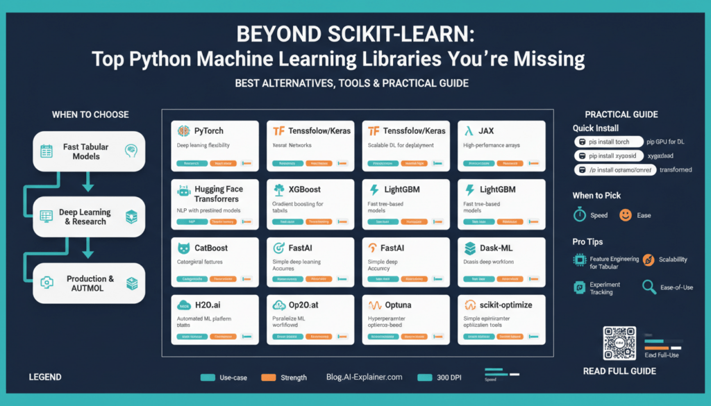
Why Look Beyond Scikit-Learn
Building on this foundation, you need to be deliberate about tool choice because Scikit-Learn was designed for a particular set of problems and workflows. If your models are classical supervised learners on tabular data, Scikit-Learn is often the fastest path from prototype to production. However, as datasets, deployment targets, and model complexity change, the limits of a single library become visible — which is why evaluating Scikit-Learn alternatives and other Python machine learning libraries early will save you rework later.
Scikit-Learn’s API shines for feature engineering, pipelines, and clean estimator semantics, but it wasn’t built for large-scale deep learning, graph models, or differentiable programming. When you need fine-grained control over backpropagation, custom loss functions, or dynamic computational graphs, frameworks like PyTorch or JAX give you primitives Scikit-Learn doesn’t expose. These frameworks enable research-driven experimentation: you can write custom autograd-friendly ops, inspect gradients at runtime, and optimize memory/compute trade-offs for GPUs and TPUs in ways that go beyond the estimator/transformer pattern.
Performance and scaling form another practical constraint. Scikit-Learn implementations are largely CPU-bound and single-process; that matches many business use cases but fails when you need distributed training, data-parallel pipelines, or inferring millions of samples per hour. For production workloads we often choose libraries that integrate with distributed compute (for example, using Dask-ML for larger-than-memory workflows or TensorFlow/PyTorch with Horovod for multi-node training). These choices reduce time-to-model for big data and make resource utilization predictable under load.
Model interoperability and deployment are common pain points that push teams beyond a single library. You may prototype in Scikit-Learn but deploy to environments that expect ONNX, TorchScript, or TF SavedModel formats; in those situations selecting a Python machine learning libraries ecosystem that supports model conversion and serving is critical. For instance, exporting a tree-based model to ONNX or switching a neural net from PyTorch to TorchServe often determines how easily you can integrate with microservices, edge devices, or serverless inference endpoints.
Another reason to diversify is algorithmic coverage: specialized problems like probabilistic modeling, causal inference, graph neural networks, or time-series forecasting frequently require libraries built for those domains. Probabilistic programming tools (e.g., Pyro, TensorFlow Probability) and graph libraries (e.g., DGL, PyG) provide algorithms, batching semantics, and evaluation metrics tailored to those tasks. Choosing domain-appropriate libraries lets you implement models more accurately and reduces the risk of misuse that arises when shoehorning domain-specific problems into generic estimators.
How do you decide when to switch? Start by asking: does my problem require custom gradients, distributed compute, specialized algorithms, or a target runtime that Scikit-Learn cannot address? If the answer is yes, adopt a hybrid stack: keep Scikit-Learn for feature pipelines and classical baselines, and use a deep learning or specialized library for the model core. For example, you might preprocess with Scikit-Learn’s ColumnTransformer and then hand off tensors to a PyTorch model for training and export. A minimal pattern looks like this:
# preprocess with sklearn
X_proc = preprocessor.fit_transform(X_raw)
# convert to torch and train
tensor = torch.tensor(X_proc).float()
model.train(); optimizer.zero_grad(); loss = criterion(model(tensor), y); loss.backward(); optimizer.step()
Adopting multiple libraries does add cognitive overhead, but it pays off by aligning tools with technical requirements. We recommend defining clear boundaries: use Scikit-Learn alternatives for model cores that need differentiation or scale, retain Scikit-Learn for reusable preprocessing and quick baselines, and standardize model interfaces across teams to simplify testing and deployment. This pragmatic, mixed-stack approach helps you move from exploratory notebooks to resilient production systems without being constrained by a single library’s assumptions.
In the next section we’ll map specific Scikit-Learn alternatives to common use cases so you can choose the right tool for your constraints and team skills. For now, accept that looking beyond one library is not about abandoning it — it’s about composing the best set of Python machine learning libraries for the job at hand.
Selecting by Task and Scale
Building on this foundation, the practical decision isn’t about finding a single silver-bullet — it’s about matching Scikit-Learn alternatives and Python machine learning libraries to the specific task and the scale you expect to run them at. How do you choose the right library when accuracy, latency, and operational cost pull in different directions? We start by defining two orthogonal axes you can use every time you evaluate a tool: the problem class (what the model must do) and the execution scale (how much data, compute, and concurrency you’ll handle). Front-loading those constraints narrows the field quickly and prevents painful rewrites later.
First, classify the problem by algorithmic needs: are you building a classical supervised estimator, a deep neural network with custom gradients, a probabilistic model that needs MCMC, or a graph algorithm that requires message-passing semantics? This classification drives your shortlist of Python machine learning libraries. For classical tabular work you’ll favor libraries optimized for gradient-boosted trees or linear models; for differentiable models you’ll gravitate to frameworks that expose autograd and low-level tensor control. Choosing by task means picking libraries that implement the right primitives rather than forcing a domain into an ill-fitting API.
Next, evaluate scale as three concrete dimensions: dataset size, training topology, and inference constraints. Dataset size influences memory strategy (in-memory vs streaming), training topology dictates whether you need single-GPU, multi-GPU, TPU, or cluster-level support, and inference constraints determine whether model size or latency is the bottleneck. These practical dimensions tell you whether a light-weight Scikit-Learn alternative is sufficient, or whether you need a framework built for distributed training and model parallelism. We recommend converting these dimensions into measurable acceptance criteria — e.g., peak throughput, acceptable tail latency, and maximum cost per prediction — and using them to reject options early.
Now map tasks to scale with concrete examples you’ll recognize from real work. If you’re iterating on feature engineering and small-to-medium tabular datasets, keep Scikit-Learn or a fast tree library in the loop for quick baselines. When you need custom backprop, image or language models, pick a deep-learning-first library that exposes autograd and device placement; this matters when you optimize mixed-precision or TPU kernels. For probabilistic inference, use a probabilistic programming library that handles sampling and variational methods; for graphs, choose a library that implements batched neighbor sampling and mini-batch training. Each choice reduces implementation friction and improves reproducibility when you match the library to the problem’s structural needs.
Scale drives operational choices as much as algorithmic ones. If you anticipate multi-node training or very large datasets, prioritize libraries and tooling with mature patterns for distributed training and data sharding; this reduces engineering debt when jobs move from experiment to cluster. In production you’ll also care about model export and serving formats — conversion to portable runtimes or optimized inference graphs can be the difference between feasible and impossible latency. Architect your pipeline so preprocessing and baseline models stay in the lightweight stack, while heavy model cores live in frameworks designed for the scale you expect.
Finally, treat selection as an incremental risk-managed process: prototype the critical path end-to-end, benchmark for your specific metrics, and measure operational costs before locking in a stack. Ask: what does reproducible training look like under failure, how quickly can we retrain, and what staff skills are required to maintain the system? By prioritizing task alignment and measurable scale requirements you’ll adopt Scikit-Learn alternatives and Python machine learning libraries for concrete reasons — reducing rework and improving deployability. In the next section we’ll map specific libraries to the common use cases you’re likely to face so you can implement the patterns we just discussed.
Deep Learning Frameworks
PyTorch, TensorFlow, and JAX are the toolset you reach for when model complexity or scale outgrew Scikit-Learn’s estimator pattern. Choose by what you need to control: do you require per-operation autograd introspection, XLA compilation for TPUs, or an ecosystem of pre-trained transformer models? When should you pick one over the others depends on the balance between research flexibility, production exportability, and hardware targets — we’ll walk through those trade-offs and practical patterns you can use immediately.
The core technical differences often determine day-to-day productivity. Autograd (automatic differentiation) lets you compute derivatives of arbitrary programs; PyTorch exposes an imperative, tape-based autograd that makes debugging and custom gradients straightforward, while TensorFlow 2 moved to eager execution with graph/Autograph options for performance. JAX takes a different approach: pure functional programming plus composable transforms (jit, grad, vmap, pmap) and XLA compilation, which yields predictable optimizations for large-scale TPU or GPU workloads. Understanding these runtimes helps you decide whether you want live-step debugging, ahead-of-time compilation, or functional transformations for parallelism.
Performance and scaling are where implementation details matter most. Mixed-precision, gradient accumulation, and optimizer-state sharding are the levers we use to train big models without changing algorithms; PyTorch’s DistributedDataParallel (DDP) and TensorFlow’s distribution strategies cover single-node multi-GPU and multi-node setups, whereas JAX’s pmap and sharded_jit map cleanly to TPU pods. For inference, export formats and accelerators (TensorRT, ONNX Runtime, TFLite) influence latency and cost; pick a framework whose export path matches your deployment target to avoid costly rewrites later.
Ecosystem and developer ergonomics speed iteration. If you want high-level training loops, Keras gives a batteries-included API for TensorFlow, while PyTorch has strong community tools like PyTorch Lightning and Ignite that standardize boilerplate without hiding control. JAX’s ecosystem (Flax, Haiku, Optax) favors explicit functional patterns and composes well with research code. For NLP and vision, Hugging Face Transformers and timm provide model zoos you can fine-tune with minimal glue, letting you focus on data and evaluation rather than reimplementing architectures.
Practical examples clarify trade-offs. If you need a custom loss that inspects intermediate activations and modifies gradients, you’ll be faster in PyTorch’s dynamic graph; write a custom autograd Function when you must override backward behavior. If you target TPUs or want to fuse ops aggressively, implement the kernel in JAX and use jit+pmap to compile a single fast executable. Here’s a minimal PyTorch custom-gradient pattern to illustrate control:
class MyOp(torch.autograd.Function):
    @staticmethod
    def forward(ctx, x):
        ctx.save_for_backward(x)
        return x.clamp(min=0)
    @staticmethod
    def backward(ctx, grad_out):
        x, = ctx.saved_tensors
        return grad_out * (x > 0).float()
Model deployment and interoperability deserve explicit planning during prototyping. Prototype in PyTorch if iterative debugging is the priority, but keep an export path in mind: TorchScript, ONNX, or a TF SavedModel (via conversion) are common production targets. For constrained devices prefer TFLite or ONNX with quantization-aware training; for low-latency server inference use TensorRT or ONNX Runtime and validate numeric parity across conversions. Designing a clear export contract — input shapes, preprocessing, and acceptable numerical drift — prevents last-mile surprises.
Building on the earlier recommendation to keep Scikit-Learn for preprocessing and baselines, compose pipelines where lightweight feature transforms remain in sklearn pipelines and the heavy model core lives in a DL runtime. For multimodal inputs, extract tabular embeddings with scikit transformers, concatenate them to convolutional or transformer representations inside the model, and perform end-to-end fine-tuning. This hybrid pattern preserves testability and reuse while giving you the gradient control you need for production-grade neural models.
As we map libraries to use cases next, keep one rule central: prototype on the platform that maximizes your velocity for the hardest part of the problem, then ensure a clean export and serving path for your chosen hardware. That discipline minimizes rework, speeds iteration, and makes the jump from notebook to scalable inference much more predictable.
Gradient Boosting Libraries
Gradient boosting remains the workhorse for structured, tabular problems where accuracy and calibrated predictions matter; when you need sharper decision boundaries than linear models and more predictable feature importance than neural nets, gradient boosting libraries are where you start. Which implementation should you pick when accuracy, training speed, and operational constraints conflict? We’ll compare practical trade-offs so you can choose by workload: prototyping speed, large-scale training, handling high-cardinality categories, or producing probabilistic outputs.
If you need raw performance and a mature ecosystem, XGBoost is often the first stop: it implements a histogram-based tree learner that’s been heavily optimized for speed and memory, and it supports CUDA-accelerated training (gpu_hist / cuda device) plus multi-GPU setups for large jobs. That GPU path lets you compress training time on large tables without rewriting your pipeline, and XGBoost’s quantile/QuantileDMatrix options help manage memory on very large datasets. (xgboost.readthedocs.io)
LightGBM targets extreme training speed with a leaf-wise (best-first) growth policy and highly optimized histogram construction; the algorithm can reach lower training loss for the same number of leaves and offers efficient categorical handling and distributed training primitives. For GPU acceleration LightGBM uses an OpenCL-based histogram builder and provides a practical path to speed up experiments across many GPU types, though you’ll want to validate GPU build compatibility and tune max_bin/num_leaves to avoid overfitting on small datasets. (lightgbm.readthedocs.io)
CatBoost differentiates itself on data ergonomics: it natively ingests categorical features and implements techniques (e.g., target-aware encodings and ordered boosting) designed to reduce target leakage and improve robustness on high-cardinality columns. If your dataset has many categorical variables and you want minimal manual preprocessing, CatBoost reduces one common source of engineering overhead and often yields competitive accuracy out of the box with fewer encoding tricks. This makes it an attractive default when you’re optimizing for developer time and repeatability. (catboost.ai)
If your problem requires probabilistic outputs rather than point predictions—predictive intervals, full conditional distributions, or proper scoring rules—consider NGBoost (Natural Gradient Boosting). NGBoost extends boosting to predict parameters of a distribution using natural gradients, so you can get uncertainty estimates directly from the model without wrapping ad-hoc calibration layers; that capability is valuable in healthcare, weather, and risk domains where decision-making needs likelihoods as inputs. (github.com)
In practice we balance three engineering constraints: data preprocessing ergonomics, computational budget (CPU vs GPU vs multi-node), and the type of prediction you need (point estimate vs distribution). For quick baselines keep Scikit-Learn for pipelines and feature transforms, then swap the model stage to an XGBoost/LightGBM/CatBoost estimator depending on your needs: XGBoost for mature GPU-accelerated training and custom quantile workflows, LightGBM for fastest leaf-wise learning at scale, CatBoost when categorical features dominate, and NGBoost when uncertainty is first-class. Tune learning_rate, early_stopping, and leaf/depth parameters while validating on a production-like holdout and measure inference latency early so export paths (ONNX, native C++ predictors, or language bindings) are clear.
Choosing between these options is a matter of constraints rather than a single ‘‘best’’ library: prioritize the hardest part of your problem. Prototype with the library that minimizes friction for that bottleneck, benchmark end-to-end on representative data, and standardize the export/serving paths so your chosen gradient boosting implementation integrates cleanly with your deployment stack and monitoring requirements.
AutoML & Productivity Tools
You waste engineering cycles when tuning the same models manually across projects; AutoML and productivity tools let you reclaim that time while keeping focus on data and evaluation. AutoML (automated machine learning) automates model selection, feature preprocessing choices, and hyperparameter optimization to produce competitive baselines quickly, and productivity tools—experiment trackers, model registries, and CI for models—help you turn those baselines into reproducible artifacts. Front-load AutoML in the first phase of experiments to reduce iteration cost, but treat its output as a diagnostic rather than a finished product. This mindset keeps velocity high without surrendering control over deployment or explainability.
Building on this foundation, AutoML is not a black box you accept blindly; it’s a rapid search mechanism that codifies best practices for model search and tuning. Define AutoML precisely on first use: it is a set of algorithms and orchestration logic that explores preprocessing pipelines, model families, and hyperparameters to maximize a chosen metric. Productivity tools complement AutoML by capturing metadata—random seeds, dataset hashes, evaluation splits—and by enabling rollback, lineage, and team collaboration. Together they reduce manual errors, enforce reproducibility, and make your experiments auditable, which matters when models move from notebook to service.
In practice you’ll use AutoML to answer concrete questions quickly: which model family suits this tabular workload, what preprocessing matters, and roughly where the accuracy/latency frontier lies? Run a short AutoML pass on a production-like holdout to identify promising architectures and then freeze a small search space for manual refinement. For example, use automated feature selection to prune high-cardinality encodings, then port the top candidates into a controlled training loop where you apply domain-specific regularization or custom loss functions. This two-stage pattern keeps the best of both worlds: rapid discovery from AutoML and fine-grained control for production-tuning.
How do you balance AutoML convenience with engineering control? The trade-offs are explicit: AutoML accelerates discovery but can obscure model internals and make hyperparameter optimization outcomes brittle if you don’t pin seeds and environment details. If you need custom gradients, explainability constraints, or strict export formats for edge devices, avoid handing the entire pipeline to an automated system. Instead, extract the promising model templates AutoML suggests, reproduce them deterministically in your preferred framework, and add tests that validate numeric parity and latency under realistic loads.
Productivity tools are where automation turns into operational reliability. Integrate experiment tracking to record AutoML trials, attach artifacts to a model registry, and enforce deployment gates via CI pipelines that run smoke tests on serialized artifacts. Use data versioning to guarantee the same feature pipeline runs in training and serving, and automate evaluation on incremental slices so you catch distribution drift early. These practices prevent the common failure mode where an AutoML-suggested pipeline performs well in a notebook but breaks during serving because of mismatched preprocessing or missing metadata.
Taking this concept further, use AutoML to shorten the feedback loop while treating productivity tools as the guardrails that make automated outputs production-ready. We recommend the pattern of discover, reproduce, and harden: discover candidates with AutoML, reproduce them deterministically in code you control, and harden with tests, monitoring, and a clear export contract. By composing AutoML with robust productivity tooling and the preprocessing patterns we discussed earlier, you convert exploratory wins into reliable, maintainable models that fit your scale and deployment constraints.
Deployment, MLOps, Interpretability
Building on this foundation, the hardest part of shipping models is rarely algorithmic—it’s the bridge between experiment and reliable production. We focus first on model deployment because a brittle export path or unclear runtime contract is what turns a successful notebook into a fire drill. You should front-load an explicit export contract (input schema, preprocessing, acceptable numerical drift) while prototyping so the later handoff to serving formats like ONNX, TorchScript, or a SavedModel is predictable. Early contracts reduce last-mile surprises and let teams reason about latency, cost, and validation before scale-up.
Treat operationalizing models as a software lifecycle with repeatable automation and guardrails rather than a one-off task. In practice that means building CI pipelines that run unit tests against serialized artifacts, a model registry to version checkpoints and metadata, and reproducible build images to guarantee parity between training and serving. Containerize the runtime (for example, Docker images that include the exact preprocessing code) and use orchestration tools for canary or blue-green rollouts so you can validate performance under realistic traffic. These MLOps practices make deployments auditable and enable safe rollback when a new model misbehaves.
Observability is the control plane for long-lived models; without it you can’t operate at scale. Instrument both prediction quality and data quality: track per-feature distributions, label skew, prediction confidence, and business KPIs tied to the model’s outputs, and surface drift as actionable alerts. We recommend coupling lightweight feature monitoring with aggregated performance metrics and example-based logging that preserves raw inputs for debugging. Observability gives you the trigger points for retraining, model rollback, or human-in-the-loop review and prevents silent degradation in production.
Interpretability isn’t a checkbox—it’s part of your feedback loop for debugging, bias detection, and stakeholder trust. Define interpretability (an explanation of how model inputs influence outputs) early and decide which form matters: global explanations (feature importance over the dataset) or local explanations (why did a model make this single prediction?). Use attribution tools—SHAP (Shapley Additive Explanations) for consistent global/local attributions and counterfactual explanations to show minimal input changes that flip predictions—so you can translate model behavior into actionable remediation steps for product and risk teams.
Integrate explainability into MLOps pipelines rather than generating reports after the fact. Automate generation of explanation artifacts at training time and persist them alongside model versions in the registry so you can reproduce why a particular model made certain trade-offs. Add explainability checks to pre-deployment gates—compare baseline Shap values, enforce invariants on important features, and flag feature-attribution shifts that could indicate data poisoning or upstream schema changes. This makes interpretability a programmatic safety net instead of a one-off manual audit.
How do you balance latency and interpretability when both matter? In latency-sensitive paths we run a lightweight surrogate (a distilled, explainable model) in front of the high-cost scorer for fast, interpretable decisions and retain the full model for asynchronous or batch scoring. For edge or constrained runtimes, export quantized models and validate that attributions remain stable under quantization; numeric parity tests should be part of the export pipeline. These patterns let you meet service-level objectives while preserving the ability to explain and debug predictions.
Finally, adopt a reproducible pattern: preprocess consistently with your training code, serialize the export with its provenance, gate deployment with automated explainability and performance checks, and close the loop with observability-driven retraining triggers. We apply this pattern across hybrid stacks—Scikit-Learn for preprocessing, a deep learning runtime for the core model, and a standardized export to the chosen serving runtime—so teams keep velocity in experimentation while maintaining production resilience. In the next section we’ll map tool choices to the common runtime targets you’ll encounter and show concrete CI/CD pipelines you can reuse.