Problem Overview and Goals
Fraud detection is a moving target: attacks evolve, legitimate behavior shifts, and the cost of getting decisions wrong is high for both users and the business. Building on this foundation, we frame the problem as simultaneously optimizing for detection accuracy, operational latency, and human review capacity—while keeping adversaries from gaming the system. You need a system that uses machine learning and deep learning where they make sense, but also respects rule-based constraints and business workflows so false positives don’t destroy conversion rates and false negatives don’t erode trust.
Our primary goals are clear and interdependent: maximize true positive capture of fraudulent activity, minimize false positives that force manual review, and sustain performance at production scale. We also require explainability for regulated contexts and fast iteration to respond to new fraud patterns. Practically, that means optimizing precision and recall in context (not just global AUC), enforcing latency SLAs for online scoring, and putting monitoring and retraining pipelines in place so models don’t degrade when behavior drifts.
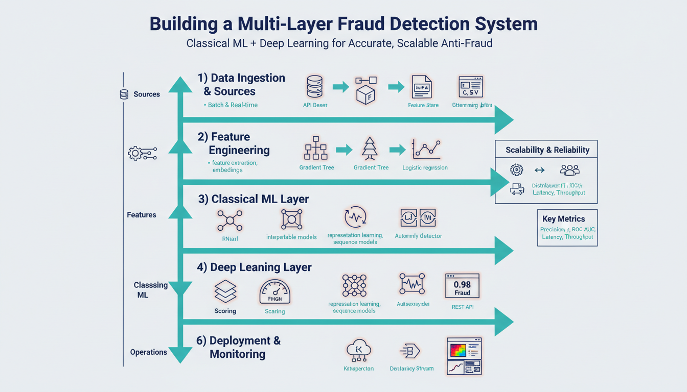
To achieve those goals we adopt a multi-layer architecture that sequences lightweight checks, classical machine learning, and deep learning models based on risk. Early layers run deterministic or fast statistical checks to stop obvious fraud and reduce load downstream. Mid layers use gradient-boosted trees or logistic regression on engineered features to provide calibrated scores for the bulk of transactions. The final layer reserves compute-heavy deep learning models—behavioral sequence models or graph neural networks—for the highest-risk cases where richer context and representation learning materially improve detection.
Data quality and labeling are the backbone of everything we do, and you must treat them as first-class engineering problems. Fraud datasets are highly imbalanced and subject to label latency, so we combine near-real-time weak labels with delayed confirmed fraud labels and keep careful lineage for each training point. Feature engineering should emphasize temporal aggregations (sliding windows, session funnels), device and network signals, and derived behavioral embeddings that feed both classical models and deep learning encoders. Also build safeguards against feedback loops where the model’s interventions change the distribution you train on.
Operational constraints determine how we choose models and deployment patterns. You’ll need a feature store for consistent online/offline features, a low-latency inferencing path for the bulk of scoring, and batch pipelines for periodic retraining and feature recomputation. Instrumenting model health—population stability, PSI, calibration drift—and business metrics like chargeback reduction and manual review rate is non-negotiable. We prioritize graceful degradation: if a deep-learning service is unavailable, the pipeline must fall back to classical ML without halting production decisions.
Evaluation must align with business impact rather than abstract metrics alone. Ask yourself: How do you balance precision and recall across layers? The answer is to cost-weight decisions using business loss models, optimize for precision at the top-k percent of risk to limit review queues, and use separate thresholds per segment (new accounts vs. long-tenured users). Track metrics such as precision@k, recall by fraud type, decision latency percentiles, and monetary savings per model version to guide deployment and rollback decisions.
Taking this concept further, our design goals translate directly into concrete architecture and ML lifecycle choices: staged scoring, targeted use of deep learning, robust data pipelines, and business-aligned evaluation. As we move into the design and implementation sections, we’ll map these goals to component-level requirements and sample patterns that you can apply to build a scalable, accurate anti-fraud system that balances automation with human oversight.
Data Collection and Preprocessing
Building on this foundation, the data you collect and the way you preprocess it determine whether your multi-layer fraud detection system will be precise and resilient or brittle and biased. Start by treating data collection as a product: instrument every event with stable identifiers, timestamps in UTC, and provenance metadata so you can trace each training example back to its source. Early choices—what telemetry you persist, how long raw logs remain immutable, and which fields are normalized at ingest—directly shape downstream feature quality and model explainability for regulated contexts. Getting these basics right reduces surprises when you push models into low-latency production paths.
Labeling is the next critical axis because label latency and weak signals are the norm in real-world fraud detection. How do you reconcile fast weak labels with delayed confirmations? We typically combine near-real-time heuristics and chargeback feeds with delayed, confirmed labels using a hybrid approach: train short-window models on weak labels for immediate responsiveness while maintaining a separate retrain schedule that incorporates ground-truth confirmations. Use label lineage and confidence scores so you can weight records during training, and consider survival-analysis framing or positive-unlabeled techniques where confirmed negatives are scarce. This balance helps contain both concept drift and the pernicious effects of label latency.
Feature engineering should prioritize temporal aggregations and behavioral context because patterns over time are where fraud signals live. Implement sliding-window and session-funnel aggregations (counts, unique devices, decay-weighted amounts) at multiple granularities—per minute for velocity checks, per day for spending behavior, per 30/90-day windows for lifetime risk. Stream-first pipelines using stateful processing let you compute incremental aggregates at scale; persist both raw events and pre-aggregated keys so you can recompute features for backfills or model audits. Derived behavioral embeddings from sequence models can feed classical models as compact representations, giving the mid-layer classifiers richer inputs without increasing online latency.
Operationalizing features requires a reliable feature store and clear operational guarantees around freshness and consistency. Push offline and online feature definitions into a shared registry so the same sliding-window logic produces identical values in training and serving, and enforce TTLs and materialized-view refresh schedules to meet latency SLAs. Serve low-latency lookups from a cache layer for bulk scoring and fall back to approximate aggregates when the store is unavailable so the pipeline degrades gracefully. Track schema changes, field deprecations, and lineage in metadata so you can replay features for any historical model version and preserve explainability.
Addressing class imbalance and avoiding feedback loops is an engineering task as much as a modeling one. Prefer cohort-aware sampling and cost-sensitive losses—class weights for gradient-boosted trees or focal loss for deep models—over naive oversampling that can amplify label noise. Keep a production holdout (shadow traffic) that does not influence automated remediation so you can measure real-world precision@k and estimate human review load without contaminating training data. When models take action, log decisions and outcomes separately so you can detect when interventions shift the population you’re training on and implement causal-aware retraining policies.
Data quality and monitoring must be continuous: set up automated checks for missingness, schema violations, psi-style population shifts, and label staleness thresholds. Instrument alerts that trigger when feature distributions or label rates diverge beyond configurable bounds, and run daily backfills of a small set of sentinel features to detect upstream regressions quickly. Preserve raw event stores for forensic reprocessing and make calibration drift metrics part of your deployment gates so we catch degrading performance before business impact accumulates.
With consistent provenance, careful handling of label latency, robust temporal aggregations, and a disciplined feature store strategy, you create a dependable substrate for the layered scoring architecture we described earlier. Next, we’ll map these prepared datasets into training pipelines and evaluation protocols that align thresholds to review capacity and business loss models, ensuring models are both accurate and operationally practical.
Feature Engineering and Representation
Building on this foundation, feature engineering becomes the gateway between raw telemetry and reliable decisions: the features you craft determine whether downstream models learn robust fraud signals or pick up brittle artifacts. Prioritize temporal aggregations and compact behavioral embeddings early—these reduce label noise sensitivity and give mid-layer classifiers high-signal inputs without blowing up latency. We’ll focus on concrete patterns you can implement and operationalize, because the right representation decides when to use classical models and when to escalate to deep learning in the final layer.
Representations should be chosen for signal-to-cost ratio: engineered aggregations (counts, uniques, velocity) are cheap and interpretable, while learned embeddings capture long-range dependencies and semantic patterns. Use engineered features for bulk scoring where you must meet strict latency SLAs, and reserve learned representations for high-risk cases or offline enrichments. This hybrid approach preserves explainability and throughput: you get calibrated scores from gradient-boosted trees and richer context from sequence-derived vectors where they materially improve precision@k.
Practical aggregation patterns are war-tested tools. Implement sliding-window aggregates at multiple granularities (1m, 1h, 24h, 30d) with decay-weighted sums for recency sensitivity and session-funnel counts to capture abandonment or rapid retries. For example, materialize online keys with SQL-like logic: SELECT user_id, COUNT(*) FILTER (WHERE success=false) AS failed_1h, SUM(amount) AS amt_1h FROM events WHERE ts >= NOW() – INTERVAL ‘1 hour’ GROUP BY user_id; use incremental stateful jobs to keep these values fresh rather than recomputing full windows. Also compute cross-device uniques and network fingerprints off the same windows so models can detect coordinated behavior without heavy joins at serve time.
How do you compress a user’s multi-session history into a compact input for a mid-layer classifier? Train sequence encoders (GRU/LSTM or a lightweight Transformer) to predict next-action distributions or reconstruct session vectors, then capture the final hidden state or a pooled representation as a behavioral embedding. Keep embeddings low-dimensional (32–128 floats), normalize them, and apply dropout or contrastive regularization during training to avoid overfitting to rare attack types. Feed these embeddings as features to a gradient-boosted tree or as auxiliary inputs to a downstream neural scorer—this gives classical models richer context without moving bulk scoring into expensive inference.
Operationalizing representations requires a disciplined feature store and determinism between training and serving. Push feature definitions into the registry so the same sliding-window logic and embedding transforms are reproducible; enforce TTLs, freshness SLAs, and a cache layer for low-latency lookups. Provide fallbacks: approximate aggregates or last-known values when the store is unavailable, and flag degraded-mode inference in logs so analysts can quantify impact. Track schema evolution and lineage so you can replay features for audits and preserve explainability in regulated workflows.
Finally, protect against leakage, bias, and feedback loops during feature construction. Use cohort-aware sampling and label-weighting to compensate for label latency, keep a production holdout (shadow traffic) that never feeds automated remediation, and log decisions and outcomes separately so you can measure how interventions change upstream distributions. Instrument PSI, calibration drift, and feature-level importance as deployment gates so we catch representation decay early. With these patterns in place, you can move clean, stable representations into the training pipelines that align thresholds to review capacity and business loss models.
Handling Class Imbalance and Augmentation
Building on this foundation, class imbalance is the single most practical hurdle you’ll face when training fraud detection models because fraudulent events are rare and heterogeneous. In fraud detection pipelines the positive class can be tiny—often well under 0.1%—so naive optimization drives models to predict “legit” and miss costly attacks. We need approaches that preserve signal from rare events without amplifying label noise, and we must treat augmentation and sampling as part of the data engineering stack, not a one-off modeling trick. Front-load class imbalance and data augmentation decisions early in your training pipeline so they propagate deterministically into production feature definitions and audits.
Start with cost-sensitive learning and cohort-aware sampling before touching synthetic data. For gradient-boosted trees use class weights or sample weights to reflect business loss (for example, set sample_weight = amount_at_risk * label_confidence), and for neural scorers use focal loss or weighted cross-entropy to concentrate learning on hard fraud examples. Cohort-aware sampling means you stratify by meaningful segments (new accounts, geographies, payment method) and upsample within segments rather than globally; that preserves joint distributions and avoids creating unrealistic examples. We also recommend positive-unlabeled (PU) techniques when confirmed negatives are scarce: treat recent weak labels differently from confirmed chargebacks by applying lower training weight and separate retrain schedules.
When you do use oversampling or SMOTE-style augmentation for tabular features, be explicit about where and why you generate synthetic records. SMOTE and its variants create convex combinations in feature space, which helps gradient-boosted models learn boundaries but can also interpolate label noise. How do you prevent synthetic augmentation from amplifying label noise? Use label confidence thresholds, restrict augmentation to high-fidelity cohorts, and validate synthetic samples on a holdout drawn from delayed-confirmation labels. Implement augmentation as a reproducible job (not an in-memory hack) and tag generated rows with provenance metadata so you can retract or reweight them if downstream monitoring flags drift.
For behavioral and sequence data, augmentation must respect temporal and graph structure: naive feature jitter destroys sequence semantics. Apply time-warping, subsequence cropping, session splicing, or contrastive perturbations on event sequences to create plausible alternate histories; when using graph-based signals, augment by negative sampling, node masking, or controlled edge rewiring that simulates realistic collusion patterns. GANs or conditional generators can synthesize rare fraud motifs for training deep encoders, but treat generated sequences as auxiliary features—never as sole evidence for automated blocking. Regularize encoders with dropout, contrastive loss, and validation on confirmed-fraud holdouts to avoid overfitting to synthetic artifacts.
Operational guardrails are as important as modeling choices. Keep a production holdout (shadow traffic) that never feeds automated remediation so you can measure real-world precision@k and review load without contamination. Log every augmentation and sampling decision in your dataset lineage; include fields for origin (real vs. synthetic), label confidence, and cohort id so retraining and audits can filter or reweight appropriately. Automate monitoring for PSI, calibration drift, and uplift by augmentation flag—if synthetic records change top-feature importance or calibration, trigger a human review and rollback path. Maintain separate retrain cadences: fast-cycle models trained on weak labels and augmented data for responsiveness, and slow-cycle models retrained with confirmed labels for calibration and governance.
Evaluate using business-aligned metrics and segment-level thresholds rather than global accuracy. Optimize precision@k for the review budget and compute monetary loss per decision to choose class weights or augmentation intensity; use backtests on historical replay to measure how augmentation changes false-positive rates in production-like traffic. Run canary experiments or A/B tests that expose augmentations incrementally and measure downstream impacts—manual review time, customer friction, and chargeback reduction—before wide rollout. Finally, surface augmentation provenance in model explanations so reviewers can understand whether a high-risk score stems from real patterns or synthetic augmentation.
Taken together, disciplined sampling, cost-sensitive losses, and carefully controlled augmentation let us amplify scarce fraud signal without amplifying noise. By treating augmentation as a reproducible, auditable component of your data pipeline and by evaluating effects on business metrics and population drift, you keep models effective and trustworthy as the system scales. Next, we’ll map these prepared datasets into training pipelines and deployment gates so thresholds align with review capacity and business loss models.
Classical Models and Stacking
Building on this foundation, classical models and stacking are the workhorses of the mid-layer where you need calibrated, fast, and interpretable risk scores. Classical models such as gradient-boosted trees and logistic regression give you high signal-to-cost returns: they run at low latency, they produce feature importances you can explain to auditors, and they integrate cleanly with the feature store and monitoring described earlier. Early placement of these models in your pipeline reduces downstream compute and keeps most decisions within tight latency SLAs while preserving the ability to escalate only truly ambiguous or high-risk cases to heavy-weight deep models.
Start by choosing models that match operational constraints and feature types. Gradient-boosted trees are excellent at heterogeneous tabular signals and handle missingness and non-linearities out of the box; logistic regression (with L1/L2) shines when you need sparsity, monotonicity, or strict explainability. Use gradient-boosted trees to absorb engineered temporal aggregates and behavioral embeddings, and use logistic regression for quick, segment-specific scoring where coefficients are business-actionable. We recommend training both on the same sliding-window feature set so their outputs are comparable and can later feed into an ensemble without costly feature transformations.
Stacking is the practical way to combine complementary classical models into a single, stronger predictor while controlling for overfitting and label latency. Stacking means producing out-of-fold predictions from base models and then training a meta-model on those predictions (and optionally a subset of original features) to learn how to weight each base learner. How do you stack without leaking temporal signals? Use time-aware cross-validation—folds that respect event times or session boundaries—so the meta-model only sees predictions that would have been available at infer time. This preserves realistic generalization and prevents the meta-layer from learning future information.
A concrete implementation pattern works well in production. First, train base learners (for example XGBoost, LightGBM, and a logistic regression) on historic sliding-window features and generate out-of-fold predictions for your training period. Persist these OOF columns into your dataset and then train a lightweight meta-model—often a regularized logistic regression or a shallow tree—on OOF predictions plus a few stable features such as account age or product type. Example pseudocode:
# train base models with time-fold CV -> produce oof_preds
# meta_X = concat(oof_preds, stable_features)
# meta_model.fit(meta_X, labels, sample_weight=amount_at_risk*label_confidence)
Train the meta-model with cost-weighting that reflects business loss so the ensemble optimizes precision@k and review capacity rather than raw AUC. Calibrate all model outputs with Platt scaling or isotonic regression per segment so thresholds translate to predictable manual-review volumes. In practice we keep per-segment thresholds (new accounts, high-value transactions) and tune them on holdout replay to align precision@k with reviewer budget and monetary loss estimates.
Operational trade-offs matter: stacking improves accuracy but increases complexity and inference cost, so we apply ensembles selectively. Route low-risk traffic to a single calibrated tree for sub-10ms scoring, and enable stacked ensemble scoring only for medium-to-high-risk transactions or in an asynchronous path that populates a cached score for near-future decisions. Monitor ensemble-specific metrics—meta-feature drift, OOF-to-production lift, PSI and calibration drift—and keep a graceful fallback path so if the meta-service is degraded you revert to the strongest single classical model. With disciplined time-aware stacking, cost-weighted meta-training, and per-segment calibration we get the detection lift classical models provide while keeping latency, explainability, and operations manageable as we escalate to richer deep-learning stages.
Deep Learning and Sequence Models
Building on this foundation, the point at which we invoke deep learning is where temporal context and long-range dependencies materially change the decision—think multi-session behavior, coordinated device hops, or evolving fraud campaigns. You want sequence models to complement, not replace, the engineered aggregations and classical models that run at millisecond latency. By front-loading this distinction we preserve throughput while directing richer, representation-learning compute only to cases where it raises precision@k enough to justify human review or automated action.
Sequence models are neural architectures that consume ordered events and produce compact behavioral embeddings that summarize a user or session history. LSTM and GRU recurrent units capture short-to-medium temporal dependencies and remain useful for moderate-length sequences; Transformers and self-attention excel when you need to model long-range interactions, variable-length sessions, or cross-session attention across heterogeneous event types. Behavioral embeddings are the fixed-size vectors we extract from these encoders—32–128 floats that capture patterns like rapid retries, device-switch motifs, or atypical navigation funnels—and we feed those embeddings into downstream classifiers to give classical models richer context without moving bulk scoring into the neural stack.
How do you train these encoders so their representations are useful in production fraud detection? Supervised sequence objectives (next-action prediction, likelihood of fraud in the next window) align representations to the business goal, while self-supervised and contrastive losses improve generalization when labeled fraud is scarce. We commonly combine short-window, weak-label objectives for high-recall responsiveness with periodic retrains on delayed, confirmed labels for calibration. This hybrid schedule preserves sensitivity to emerging attacks while keeping calibration and governance intact for regulated decisions.
In practice you’ll implement an encoder that maps event tokens (type, amount bin, result, device hash) plus positional/temporal features into a pooled vector, then persist that vector to the feature store for downstream use. Example PyTorch pseudocode shows the minimal flow:
# seq: [batch, seq_len, feat_dim]
encoder = TransformerEncoder(d_model=64, n_heads=4, layers=2)
hidden = encoder(seq)
embedding = hidden.mean(dim=1)  # pooled behavioral embedding
# persist embedding to feature store, or pass to a GBDT
Keep the embedding pipeline deterministic and versioned so the same encoder behavior is reproducible between offline training and online serving. In scoring, you’ll rarely call a heavy encoder for every request: route only medium-to-high risk transactions to the neural service, cache recent embeddings per account/session, and compute asynchronously where possible so latency SLAs for bulk traffic remain under control.
Operational constraints shape model architecture and serving patterns. Deploy encoders behind a scalable inference service with autoscaling and GPU pooling for batch encoding; expose a fast gRPC path for cached lookups and an async path that writes a risk-score back into a results cache. Provide a graceful fallback to the calibrated classical model when the neural service is degraded. For explainability, wrap attention weights or integrated gradients into surrogate explanations and expose those alongside calibrated scores so reviewers and auditors can inspect why a sequence model flagged an event.
Robustness and governance need equal attention: avoid temporal leakage by using time-aware folding and never training on events that wouldn’t have been available at inference time. Regularize encoders with dropout, contrastive augmentation, and validation on confirmed-fraud holdouts to prevent overfitting to synthetic patterns. Monitor embedding drift (PSI on embedding dimensions), calibration drift, and uplift metrics (precision@k, manual review load) and include embedding-origin metadata (real vs. synthetic, label confidence) in lineage so you can trace and roll back problematic retrains.
Taken together, sequence models and deep learning give us a powerful final-layer capability: they convert messy temporal histories into compact, high-signal behavioral embeddings that elevate precision where it matters. Next we’ll connect these encoders to graph-based enrichments and operational deployment gates so the system scales without sacrificing explainability or SLA guarantees.
Evaluation, Monitoring, and Deployment
Fraud detection systems live or die on their operational feedback loop: how you evaluate model decisions, continuously monitor health, and deploy updates determines whether detectors catch new attacks or quietly degrade into noisy blockers. How do you align evaluation with business impact so review queues and chargebacks move in the right direction? We’ll show pragmatic, production-focused patterns for evaluation, model monitoring, and safe deployment that map directly to the layered architecture and feature-store guarantees we discussed earlier.
Start evaluation with business-aligned metrics rather than global AUC: optimize precision@k where k equals your reviewer capacity and cost-weight thresholds by monetary exposure per decision. Precision@k focuses measurement on the top-ranked alerts you will actually act on, which makes it the right objective when your manual-review budget is the gating constraint and when you must tune per-segment thresholds (new accounts, high-value transactions). Use precision@k together with cost-weighted sample weights in training so optimization directly reflects business loss and review capacity. (oecd.ai)
Monitoring must detect the kinds of drift and failure modes that matter: population shifts in inputs, calibration drift in scores, embedding drift for learned representations, and operational regressions like latency or error spikes. Compute univariate and score-level stability metrics (for example, Population Stability Index on features and scores) and treat them as alerts that trigger investigation or automated rollback when breaches are persistent. Also instrument model-agnostic detectors that flag likely performance deterioration without labels—for example, ensemble disagreement or statistical detectors on predictive distributions—so you can surface failures even when confirmed fraud labels lag. These signals help prioritize retrains and forensic label-collection. (mdpi.com)
Instrumenting health means more than dashboards: log decisions, inputs, feature snapshots, model version, and label lineage for every flagged item so you can replay, audit, and compute delayed-ground-truth metrics. Maintain a production holdout (shadow traffic) and a labeled backlog to estimate true precision@k and calibration after label confirmations, and expose degradation gates that combine PSI, calibration error, and business KPIs (chargeback rate, review throughput) before allowing automated remediation. Flag degraded-mode inference in every decision record so analysts can quantify business impact when fallbacks are active.
Deploy with staged rollouts and resilient fallbacks so model updates don’t create outage or unacceptable user friction. Use canary or blue/green patterns to ramp new versions (start 1–5% traffic, monitor infra SLOs and proxy KPIs, then increase) and keep the previous model warm for instant rollback; run shadow deployments in parallel to validate predictions without affecting outcomes. Provide a deterministic, low-latency fallback path (the calibrated classical model or deterministic rules) so an encoder or heavy service outage gracefully returns a safe score rather than blocking decisions. Automate rollback runbooks and guardrails in your CI/CD pipeline so latency spikes or KPI regressions trigger immediate remediations. (docs.aws.amazon.com)
Finally, tie monitoring to retraining and deployment cadence: treat short-cycle models trained on weak labels as exploratory and require periodic re-calibration with confirmed labels; gate full promotion on holdout replay and canary performance on precision@k and calibration error. Version models, feature definitions, and embedding encoders in a registry, and automate promotion only when lineage, PSI, and business KPIs pass thresholds. Taking this approach lets you iterate quickly on emerging attacks while ensuring each rollout is auditable, reversible, and aligned with reviewer capacity—so the system improves detection without increasing customer friction or operational risk.