What Is a Vector Database
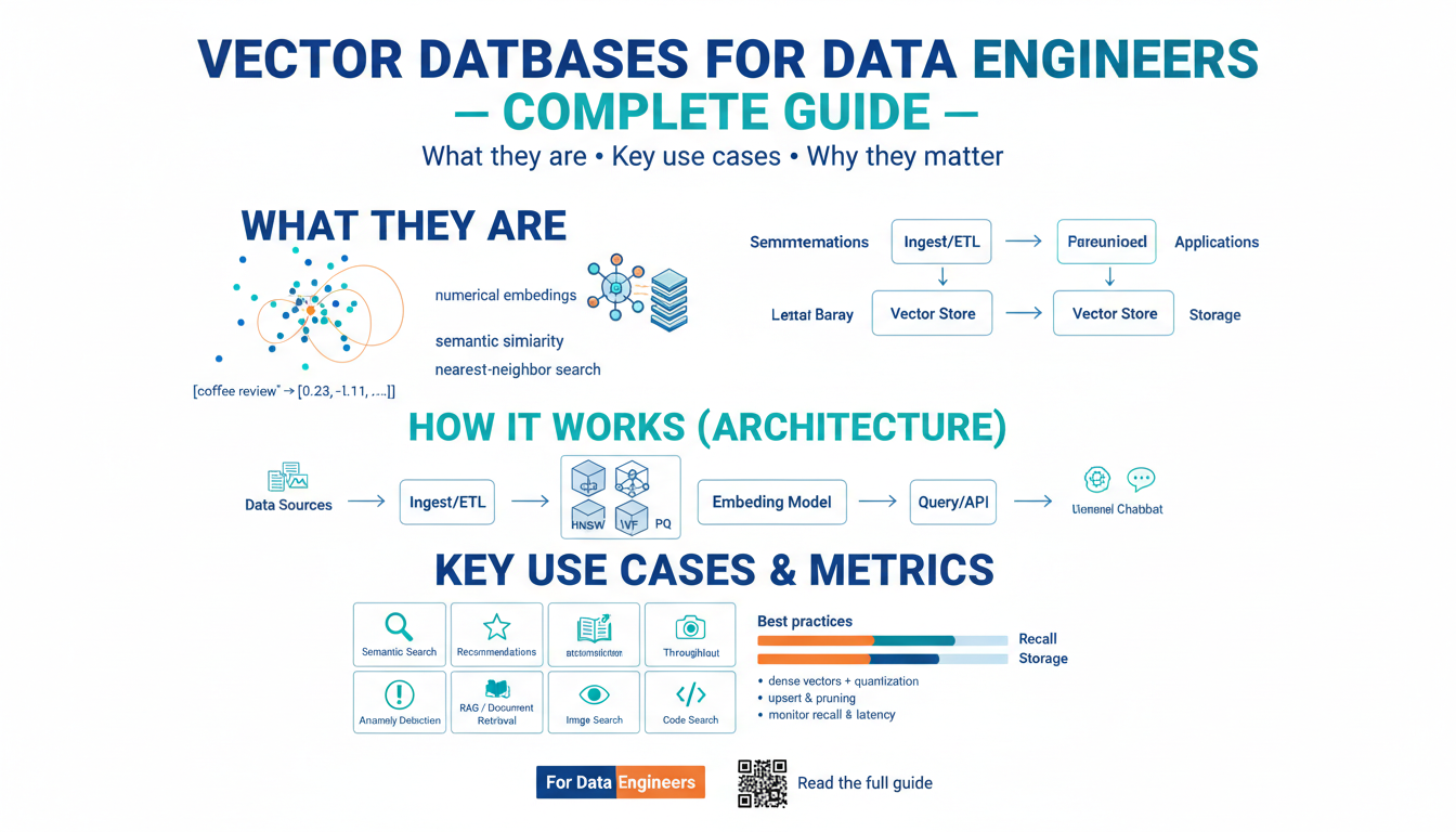
Building on this foundation, imagine searching by meaning instead of exact text matches — that’s the core purpose of a vector database and why vector search has become central to modern ML-driven applications. A vector database stores numeric vectors (dense arrays of floating-point numbers) that represent semantic embeddings — compact numerical representations of unstructured data produced by models. Embeddings capture meaning so that semantically similar items are close in vector space, and a vector database optimizes for similarity queries (nearest neighbors) rather than relational joins or transactional updates.
At a high level, a vector database contains three primary parts: the vector payload (the embeddings), associated metadata (IDs, raw text, timestamps, application-specific fields), and an index optimized for similarity search. The index is usually an approximate nearest neighbor (ANN) structure that trades a small amount of recall for large gains in query latency; common algorithms include HNSW (Hierarchical Navigable Small World graphs) and quantized product-quantization approaches. You’ll also see APIs to upsert vectors, fetch top-K neighbors with distances, and filter results using metadata predicates to combine semantic and structured filters.
Why is this different from a conventional database? Traditional databases answer equality or range queries on structured columns; they aren’t built to answer “which documents are semantically closest to this query?” A vector database computes similarity using metrics like cosine similarity, Euclidean distance, or inner product and uses vector neighborhoods as the retrieval primitive. This makes vector databases ideal for semantic search, recommendation, and retrieval-augmented generation where meaning and similarity override exact keyword matches.
In practice you build a simple ingestion pipeline: normalize raw inputs, call an embedding model, and persist both vector and metadata into the vector store. For example, a minimal ingestion pattern looks like this:
text = "Customer support ticket about login failure"
vec = embed_model.encode(text)        # produces a float32 array
vec = normalize(vec)                  # optional: L2-normalize for cosine
db.upsert(id=uuid(), vector=vec, metadata={"text": text})
This pattern lets you separate concerns: model selection and vector generation remain independent from the storage/indexing strategy, so you can swap embedding models or reindex without rewriting downstream logic.
Operational trade-offs matter. ANN indexes like HNSW provide sub-10ms latency at high recall for many use cases, but memory consumption and index rebuild times grow with dataset size. Quantization (e.g., product quantization) reduces memory at the cost of slightly lower recall. Sharding strategies, persistent-storage options, and asynchronous batch-updates affect write latency and freshness; if you need frequent writes and low-latency reads, plan for incremental indexing or hybrid architectures that combine in-memory hot stores with disk-backed cold shards.
Real-world applications make these choices concrete. Use semantic search when users expect concept-level matches across documents; power recommendation systems by computing similarity between user embeddings and item embeddings; enable retrieval-augmented generation (RAG) by returning relevant passages for a language model to condition on. In fraud detection and anomaly hunting, embedding behavioral sequences lets you group similar patterns quickly. In each scenario, keep metadata close to vectors so you can apply deterministic filters or enrich results for downstream business logic.
How do you evaluate whether a vector database meets your needs? Measure recall@K and precision for your retrieval tasks, track end-to-end latency and QPS, and test impacts of index parameters (efConstruction, M for HNSW, PQ bit widths) on both accuracy and throughput. Monitor update patterns, storage costs, and operational complexity; often the right answer is a hybrid: an OLTP datastore for authoritative records plus a vector database for semantic retrieval.
Taking this concept further, next we’ll look at concrete integration patterns and when to choose an embedding model, index type, and deployment topology for production workloads. That will help you move from understanding what a vector database does to deciding how to operate one at scale.
How Embeddings Represent Your Data
Building on this foundation, think of embeddings as the language your data speaks inside a vector database: numerical fingerprints that encode semantics, context, and task-specific signals so you can search by meaning rather than exact text. Early in the pipeline we convert raw tokens into dense vectors, but the real design choices come after encoding — how you chunk text, whether you normalize vectors, and how you pair vectors with metadata all shape retrieval quality for semantic search and downstream tasks. We’ll treat embeddings as actionable engineering artifacts, not black-box outputs from a model, and show practical patterns you can apply immediately.
At a conceptual level, an embedding is a point in high-dimensional geometry where proximity implies semantic relatedness. Models imprint training signals (language modeling, contrastive objectives, supervised labels) onto vector directions, so similar concepts cluster and dissimilar ones separate. This is why sentence-level embeddings differ from token-level or passage-level embeddings: the model’s receptive field and objective determine whether a vector represents a phrase, a paragraph, or an entire document. When you choose an embedding model, decide which semantic granularity matches your queries — fine-grained intent detection needs denser, shorter-span vectors, while topical retrieval benefits from aggregated passage embeddings.
Practical numeric choices matter because they change how the vector database evaluates similarity. Normalize vectors (L2-normalize) if you plan to use cosine similarity, because cosine(u,v) equals the dot product when vectors are on the unit sphere; skip normalization if your index expects raw inner products and you’ve calibrated the model accordingly. Dimensionality affects expressivity and cost: higher dims can capture subtler semantics but increase index size and ANN search latency; quantization reduces memory but adds approximation error. How granular should your embedding be for a given retrieval task? Test recall@K and downstream utility (e.g., RAG answer accuracy or click-through for recommendations) on representative queries to find the sweet spot between vector dimensionality, chunk size, and index configuration.
Chunking and pooling choices determine what each vector actually represents in practice. For long documents we typically split into overlapping passages (for example 200–500 tokens with 50–100 token overlap) so a single semantic query can match localized context instead of diluting meaning across the whole document; for short items you may embed the entire record. Pooling strategies matter too: CLS-token embeddings, mean pooling of token vectors, or learned pooling heads produce different geometric properties and retrieval behavior. In recommender or deduplication flows, embedding individual attributes (title, description, user activity sequences) and then concatenating or averaging vectors can yield better signals than a single monolithic embedding.
Operationally, embeddings evolve: models get updated, user behavior drifts, and new content changes neighborhood topology. Plan for re-embedding cadence (hot items on write, periodic full reindexing, or lazy re-embed on first access) and track embedding drift metrics such as shift in average pairwise cosine distributions. Ensure your vector database metadata and filter predicates remain authoritative so you can combine deterministic rules with semantic neighbors. We also recommend A/B testing alternative embedding models or chunking heuristics and measuring end-to-end metrics (latency, recall@K, and business KPIs) rather than only vector-space statistics.
These representation decisions have downstream consequences for index choice, latency, and model selection, so treat embeddings as part of your system design rather than an afterthought. When we choose dimensionality, normalization, chunking, and re-embedding strategies with empirical tests, the vector database becomes a predictable, maintainable component of your stack. Next we’ll map these representation patterns to concrete integration choices — which embedding models to pick, which ANN index parameters to tune, and how to deploy a hybrid storage topology for production workloads.
Indexing and Approximate Nearest Neighbor
Building on this foundation, the single most important engineering decision for retrieval performance is the index that sits alongside your vector database — specifically the choice and configuration of an approximate nearest neighbor (ANN) structure that will serve high-throughput similarity search. How do you pick the right index for your workload? We’ll walk through the operational trade-offs you’ll tune for production: recall versus latency, memory footprint versus accuracy, and updateability versus query throughput.
At a conceptual level, ANN algorithms trade a small amount of recall to avoid O(N) brute-force scans. Instead of exhaustively comparing a query vector to every stored vector, ANN algorithms generate a candidate neighborhood using graph, tree, or quantization structures and then return top-K neighbors with high probability. This approximation is intentional: it lets you hit millisecond latencies at large scale while using similarity metrics such as cosine similarity, Euclidean distance, or inner product. Understanding the specific failure modes — missing tail examples, sensitivity to dimensionality, and metric miscalibration — helps you decide whether an approximate index is acceptable for a given use case.
A common practical choice is HNSW (Hierarchical Navigable Small World). HNSW constructs multi-layer proximity graphs that let queries descend from coarse to fine neighborhoods, delivering excellent recall-latency trade-offs for many semantic search and recommendation workloads. Two control knobs you’ll tune are M (the maximum number of neighbors per node) and efConstruction (the effort spent while building the graph); larger M and higher efConstruction increase recall and robustness at the cost of memory and build time. At query time efSearch controls search breadth; raising efSearch improves recall but increases per-query CPU. We recommend iteratively tuning these parameters with a representative query set and tracking recall@K and p95 latency rather than guessing values.
When memory is the bottleneck, product quantization and other vector-compression techniques become essential. Product quantization (PQ) splits vectors into subvectors and compresses each subspace with a codebook, drastically reducing storage while enabling fast asymmetric distance computations. The trade-off is quantization error: PQ will reduce recall compared to full-precision indexes. A common engineering pattern is hybrid retrieval: use a compressed index (IVF+PQ or PQ-only) for candidate generation at billion-scale, then rerank the top candidates against stored full-precision vectors or recomputed distances to restore accuracy for the final K results.
Index lifecycle and write patterns shape architecture choices. If your workload requires frequent inserts and near-real-time reads, favor indexes that support incremental updates or maintain a small in-memory write buffer that flushes into a background rebuild. For append-heavy systems we often run a hot in-memory shard for recent items and cold, compacted disk-backed shards for older data; periodic background merges reconcile them. Sharding by semantic partition (for example, user segment or vertical) helps keep individual index sizes manageable and reduces the impact of reindexing. Keep metadata tightly coupled with vectors so you can apply deterministic filters before or after ANN candidate selection to combine semantic and structured predicates efficiently.
Measure what matters: recall@K on realistic queries, p50/p95/p99 latencies, QPS, memory per shard, and index build time. Use offline benchmarks that reflect your production query mix and also run shadow traffic to validate changes under load. When you tweak an index parameter, capture both retrieval quality and system cost; small recall gains rarely justify large memory or latency penalties. Taking these experiments together, you can select an index topology — HNSW for low-latency, high-recall needs; IVF+PQ for massive-scale storage efficiency; or hybrid designs that combine both — and then iterate based on empirical metrics as your corpus and query patterns evolve.
Next we’ll map these index trade-offs to embedding choices and deployment topology so you can pick models and operational patterns that align with your latency, cost, and freshness requirements.
Building Ingestion Pipelines and Transformations
Building on this foundation, the first practical problem we tackle is how to move raw data into a vector database reliably and observably. An ingestion pipeline is the bridge between source systems and embeddings: it normalizes inputs, applies deterministic transforms, calls an embedding model, and persists vector + metadata. How do you design that pipeline so it’s resilient to schema drift, model updates, and bursty traffic? Asking that up front forces decisions about batching, idempotency, and observability that determine long-term maintainability.
Start by defining a stable canonical record for each item you’ll embed; this schema becomes the contract between producers and the rest of the stack. Normalize text, remove PII when required, and extract structured attributes you’ll use as metadata filters in queries. We recommend generating a content-hash (e.g., SHA-256 over normalized text) and storing it with each row so your pipeline can detect duplicates, skip re-embeds, and perform idempotent upserts to the vector store. This single-source-of-truth approach reduces accidental drift when you rotate embedding models or change chunking rules.
Batching and streaming are complementary ingestion patterns; pick both deliberately based on freshness and throughput needs. For high-throughput bulk backfills or re-embedding jobs, use controlled batches that parallelize embedding calls and then perform bulk upserts to the vector database to amortize overhead. For near-real-time freshness, run a streaming pipeline (e.g., Kafka or a serverless event bus) that does lightweight validation and sends small, frequent embedding requests; combine that with a write buffer or hot in-memory shard to avoid degrading ANN index performance from constant small writes. Tuning batch size and concurrency is critical: too small and you blow I/O costs; too large and you risk model-rate limits and high memory pressure.
Transformations between raw text and stored vectors deserve operational telemetry and test coverage like any other critical service. Implement deterministic chunking rules (for example, 200–400 token windows with overlapping context) and unit-test them against edge cases like tables, long lists, and code snippets so chunk boundaries don’t drop important context. Normalize and optionally L2-normalize embeddings based on your similarity metric decisions, and record vector statistics (mean norm, dimensionality checks, pairwise similarity histograms) to detect embedding drift. Instrument pipelines to emit metrics for input throughput, embedding latency, downstream upsert latency, and rejection/error rates so you can correlate retrieval regressions with upstream changes.
Practical engineering includes safeguarding costs and correctness during model evolution and reindexing. When rolling a new embedding model, run a shadow re-embed on a representative subset and compute retrieval metrics (recall@K, rank correlation) before switching readers to the new index. For full reindexes, stream a staged migration: create a new index, bulk-load re-embedded vectors, run A/B traffic split for semantic search queries, and monitor production KPIs. Maintain metadata that links vectors to source IDs and embedding model versions so you can roll back or selectively re-embed failed partitions without touching the entire corpus.
Finally, make pipelines observable and automatable so they support the lifecycle you need: ingestion, validation, re-embedding, and retirement. Capture lineage (source file, transform steps, model version) alongside each vector so you can answer “why did this document change neighborhoods?” in production. As we discussed earlier, representation and index choices interact closely, so instrumenting your ingestion pipeline lets you iterate on chunking, normalization, and embedding cadence with measurable impact. Next we’ll translate these operational patterns into index and deployment choices so we can close the loop between how vectors are produced and how they’re searched.
Common Production Use Cases Explained
Building on this foundation, production systems use vector databases to turn semantic relationships into reliable application behavior rather than experimental prototypes. If your users expect meaning-aware results, you’ll deploy semantic search and similarity retrieval as first-class features that must meet SLAs for latency, recall, and freshness. In practice that means pairing well-chosen embeddings with an ANN-backed index and operational controls for write patterns, metadata filters, and reranking. We’ll walk through the production patterns you’ll see most often and how to make pragmatic trade-offs between quality, cost, and responsiveness.
One of the most common deployments is semantic search over documentation, support tickets, and knowledge bases. In those flows you embed passages or FAQ answers and store the dense vectors alongside authoritative metadata so you can apply deterministic filters before or after nearest-neighbor lookup. For example, supporting an enterprise search where results must obey tenant boundaries requires combining vector similarity with exact-match predicates (tenant_id, doc_version), and reranking the top candidates with BM25 or a cross-encoder to restore precision. This hybrid approach leverages a vector database for recall while preserving auditability and deterministic rules for compliance-sensitive use cases.
Recommendation and personalization are another high-impact production pattern. We typically compute user and item embeddings from behavioral signals (click sequences, purchases, content features), then score candidate items by vector similarity and business heuristics. In an e-commerce recommender you might generate a candidate set with ANN, apply business filters (inventory, regional availability), then rerank by predicted CTR using a gradient-boosted model. Address cold-start by mixing content-based embeddings with collaborative signals and maintain real-time personalization via a hot in-memory shard for recent activity while the cold index is compacted on disk.
Retrieval-augmented generation (RAG) architectures illustrate how vector retrieval becomes a dependency for LLM-driven features. In RAG you fetch top-K passages with a vector database and pass them as context to the generator; quality hinges on chunking strategy, embedding granularity, and ANN recall. How do you prevent irrelevant context or hallucinations? Use conservative candidate generation (higher efSearch for HNSW), rerank with a cross-encoder or recalled exact-match checks, and include provenance metadata in the prompt so the model can cite sources. For latency-sensitive assistants, consider asynchronous reranking or a two-stage pipeline: cheap ANN candidate generation followed by a smaller set of expensive re-evaluations.
Beyond search and recommendations, vector stores power anomaly detection, deduplication, and intent clustering in production telemetry and fraud systems. Embedding user sessions, API call sequences, or transaction vectors lets you surface near-duplicate attacks, detect pattern drift, and group behavior semantically faster than rule-based heuristics. Operationally this means instrumenting re-embedding cadence, running streaming ingestion for hot events, and sharding by semantic partitions (region, product line) so tail queries and reindexes don’t degrade cluster performance. Maintain lineage and model-version metadata so you can trace why a suspicious cluster appeared and roll back embeddings if needed.
Finally, treat these use cases as engineering projects: define metrics (recall@K, p95 latency, QPS), automate A/B tests for embedding/model changes, and build observability for vector-space health (norm distributions, nearest-neighbor stability). Tune ANN and index strategies to match each use case—HNSW for low-latency high-recall features, PQ/IVF hybrids for cost-constrained billion-scale corpora—and combine in-memory hot stores with compact cold shards to balance freshness and cost. In the next section we’ll map these use cases to concrete decisions about embedding model selection, index parameters, and deployment topology so you can implement production-ready vector retrieval with predictable behavior.
Deployment, Scaling, Monitoring, And Costs
Building on this foundation, the hard part of making a vector database production-ready is operational: how you deploy, scale, monitor, and control costs while preserving recall and latency. We often start with a single question: how do you deliver millisecond semantic search and high-QPS similarity without bankrupting the project? Answering that requires tying your index choices (HNSW, IVF+PQ, etc.), storage topology, and deployment strategy to concrete SLOs and traffic patterns rather than guessing on resource allocations.
Choose deployment topology based on update patterns and hardware constraints. For read-heavy, near-real-time semantic search, a hot in-memory shard that holds recent vectors and an SSD-backed cold layer for older vectors works well; the hot shard keeps p95 latency low while the cold layer reduces RAM costs. If you self-host, use Kubernetes StatefulSets for stable node identity and persistent volumes (NVMe-backed SSDs for index IO), and expose metrics via sidecars. Managed vector database offerings remove orchestration overhead but shift choices to provisioning and multi-tenant isolation, so compare latency guarantees and data locality when evaluating providers.
Scaling is a mixture of architecture and knobs. Horizontal sharding by semantic partition (tenant, region, or vertical) keeps per-shard index sizes manageable and reduces rebuild blast radius, while replica sets improve read throughput and availability. For ANN-specific scaling, tune efSearch and M on HNSW to trade latency for recall under load; if you hit memory limits, move candidate generation to a compressed index (IVF+PQ) and rerank top candidates with full-precision vectors. Autoscale CPU and memory for query nodes but avoid aggressive autoscaling for index builders—index construction is I/O and memory intensive and benefits from steady capacity.
Monitoring and observability must include both system and vector-space signals. Track p50/p95/p99 query latencies, QPS, error rates, index build time, and memory per shard, and pair those with vector-space telemetry like recall@K on a synthetic query set, nearest-neighbor stability, and distribution of cosine similarities (to detect embedding drift). Run shadow traffic for config changes and use synthetic warmup queries after deployments to populate caches. Alert on rising index build times, sudden drops in recall@K, or shifts in mean vector norm; those are early indicators that a re-embed, reindex, or model rollback may be necessary.
Costs are often the deciding constraint; RAM and NVMe are the biggest drivers for large vector stores. Reduce costs by combining techniques: product quantization or OPQ for storage reduction, tiered storage (RAM for hot shards, SSD for warm, object storage for archive), and candidate pre-filtering using deterministic metadata to avoid unnecessary ANN work. Batch upserts and throttle reindex jobs to avoid repeated full rebuilds. Remember the trade-offs: PQ and quantization save money but add approximation error, so compensate with a reranking step for the final K results when accuracy matters.
Operational practices tie everything together: automate index builds and migrations in CI/CD pipelines, maintain model-version metadata for each vector, and use blue/green or canary reindexing so we can compare retrieval quality before switching traffic. Regularly snapshot indexes and verify restore procedures to meet your RTO/RPO. As you iterate, map observed costs and SLO violations back to index parameter choices and embedding cadence so you can make predictable decisions about model updates and deployment topology in the next phase where we choose embedding models, index parameters, and topology to match your SLAs.


