Decision Trees: Basic Concepts
Building on this foundation, we’ll unpack the core mechanics that make decision trees effective for both classification and regression tasks. At their heart, a tree is a sequence of binary or multi-way splits that partition the feature space into regions with homogeneous targets; leaves represent final predictions. You should think of a tree as a set of if/then rules that are learned from data rather than hand-crafted, which is why trees are intuitive for debugging and communicating model behavior. Early on we trade-off simplicity and fit—understanding that trade-off is central to using trees well.
A split is chosen to maximize a reduction in impurity, so understanding impurity measures is essential. Entropy and Gini impurity (for classification) and variance reduction (for regression) are the usual criteria; entropy quantifies the unpredictability in a node and information gain is the parent impurity minus the weighted child impurity. How do you pick the best split? In practice you evaluate every candidate threshold (for continuous features) or partition (for categorical features) and pick the one with highest information gain or greatest variance reduction, often using efficient algorithms that scan sorted feature values. Implementationally, this is why sorting numeric columns and caching split statistics dramatically speeds training.
Controlling model complexity prevents overfitting, so explicit stopping rules and pruning must be part of your workflow. Maximum depth, minimum samples per leaf, and minimum impurity decrease are direct hyperparameters you can tune; post-hoc pruning (cost-complexity pruning) removes branches that don’t improve generalization according to a validation criterion. In real-world datasets—imbalanced fraud detection or noisy sensor streams—unrestrained trees memorize outliers and produce brittle rules, so we prefer moderate depth and validate with cross-validation or a holdout set. Regularization via pruning or constraints also reduces variance and improves the stability of feature importance estimates.
Trees handle different feature types and missing values, but choices matter for performance and interpretability. For continuous variables you create numeric thresholds (e.g., feature > 42.7); for categorical variables you can use one-hot encoding, target/impact encoding, or native multi-way splits depending on cardinality and implementation. Many production tree libraries offer built-in missing-value handling through surrogate splits or default directions; when they don’t, imputation or a dedicated missing indicator preserves signal. Practically, we often encode high-cardinality categories with target statistics or hashing to avoid explosive branching that harms both speed and generalization.
Interpretability is a major strength, but you should quantify and validate explanations rather than assume clarity equals correctness. You can trace a prediction to a path of conditions and produce human-readable rules like “if income > 80k and credit_score < 650 then risk = high,” which is immediately actionable for stakeholders. For more robust explanations compute feature importance (split-based or permutation-based) and complement it with partial dependence or SHAP values when interactions matter; be aware that raw split counts can be misleading on correlated features. Also evaluate fairness and stability of rules—small data shifts can flip paths and change decisions, so unit tests on example cases and monitoring in production are essential.
Now that we’ve established how nodes, splits, impurity, and pruning interact in practice, the next step is to implement these ideas and tune hyperparameters on real data. In the implementation section we’ll translate impurity calculations into efficient code, demonstrate pruning strategies, and show common pitfalls with categorical encoding and missing values. By focusing on the why and the when—rather than only the how—you’ll be better positioned to select the right tree configuration for classification or regression problems and to move confidently into ensemble methods that build on these basics.
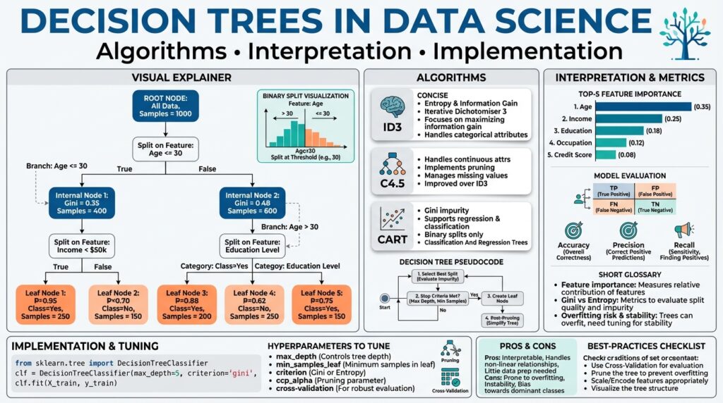
Core Algorithms: ID3, C4.5, CART
Building on this foundation, let’s examine the classic tree induction recipes you’ll actually implement and tune in practice: ID3, C4.5, and CART. Each algorithm encodes a different set of assumptions about impurity, split structure, handling of continuous features, and pruning—so understanding those differences clarifies why one algorithm produces shallower, multi-way trees while another yields binary trees optimized for ensembles. We’ll reference entropy, information gain, Gini impurity, and variance reduction that you already met, and show concrete trade-offs you’ll face when training decision tree models on real datasets.
ID3 is the simplest of the three and is useful to reason about because it makes explicit the information-theoretic view of splitting. The core idea is to pick the attribute that maximizes information gain (reduction in entropy) at each node; entropy measures the unpredictability of class labels and information gain ranks candidate splits accordingly. ID3 originally assumed categorical attributes and did not include robust pruning or native handling of continuous features, so in practice you either discretize numeric columns or move to C4.5/CART for richer feature sets. Use ID3 when you want a clear, interpretable baseline and when your features are mostly low-cardinality categorical variables.
C4.5 evolved from ID3 to address practical shortcomings you’ll encounter in applied workflows. It introduces continuous attribute thresholds by searching sorted values for best split points, applies the gain ratio (information gain normalized by split information) to avoid bias toward high-cardinality attributes, and implements handling for missing values via fractional instance assignment. Crucially, C4.5 adds post-pruning based on estimated error rates (confidence-based pruning), which reduces overfitting on noisy training data. When your dataset mixes numeric and categorical features, and you care about a single-tree interpretable model with built-in pruning, C4.5 is a strong choice.
CART (Classification And Regression Trees) takes a different path that matches modern pipeline needs like ensembling and regression tasks. CART uses Gini impurity for classification and variance reduction for regression, and it enforces binary splits—every internal node gives two children—making the tree structure simpler and often faster to evaluate. The algorithm produces piecewise-constant predictions at leaves and uses cost-complexity pruning (the alpha parameter) to trade off fit versus tree size; this pruning strategy is easy to cross-validate because you can compute the complexity parameter path and select the alpha that minimizes validation error. If you plan to build random forests or gradient-boosted trees, CART-style binary splits and impurity measures align naturally with those ensemble methods.
How do you decide which algorithm to choose for your dataset? Prefer C4.5 when you need native support for mixed attribute types, missing values, and multi-way splits with a single interpretable tree; choose CART when you want regression support, binary splits that play well with ensembles, or when you need explicit cost-complexity pruning. ID3 is useful pedagogically and as a minimal baseline but typically gives way to the more practical C4.5/CART implementations in production. Evaluate via cross-validation on metrics relevant to your domain—AUC for imbalanced classification, RMSE for regression—and inspect tree depth and leaf sizes to avoid brittle rules.
In implementation, the same efficiency tactics you learned earlier apply: sort continuous features once and scan thresholds, cache class histograms to compute impurity deltas in O(1) per candidate, and use parallel evaluation of features when you have many columns. For missing values and production robustness, CART’s surrogate splits let you find secondary features that mimic a primary split behavior, which preserves decision logic when values are absent—this yields more stable, auditable rules than blanket imputation. For categorical features with high cardinality, consider grouping by target statistics or using target encoding before feeding a tree algorithm to avoid combinatorial partitioning that harms both C4.5 and CART.
In practice, tune pruning and split-stopping rules aggressively: set sensible min samples per leaf, minimum impurity decrease, or the cost-complexity alpha to constrain growth. Measure feature importance stability under bootstrap resamples to catch spurious splits caused by correlated predictors. By matching the algorithm (ID3/C4.5/CART) to your data characteristics—feature types, missingness pattern, need for regression support, or ensembling—you’ll choose the right decision tree foundation and avoid common pitfalls that turn interpretable models into overfit artifacts.
Splitting Criteria and Impurities
Choosing the right split at a node determines whether a tree generalizes or memorizes noise, so we need to treat splitting criteria and impurity measures as design decisions, not defaults. In practice you’ll choose between entropy (information gain), Gini impurity, or variance reduction depending on your task and downstream metric, and you should evaluate how those choices interact with class imbalance, categorical cardinality, and runtime constraints. How do you decide which impurity to prefer for a given problem? Below we unpack the practical trade-offs and concrete patterns you’ll use when implementing and tuning trees.
Entropy and Gini both aim to create purer child nodes, but they behave slightly differently in ranking candidate splits, which matters in edge cases. Entropy (information gain) has an information-theoretic basis and can be more sensitive to changes near class-probability extremes; Gini tends to prefer splits that isolate the largest class quickly. For most classification tasks Gini and entropy yield similar trees, but when you have high-cardinality categorical features or skewed classes, entropy’s sensitivity and Gini’s computational simplicity lead to different split orders—so compare both on a validation metric rather than assuming one is universally superior.
For regression tasks we work with variance reduction (equivalently mean squared error decrease) as the impurity objective, and the implementation pattern is straightforward: sort a numeric feature, maintain running sums and squared sums, and compute left/right variance in O(1) per threshold. A practical pseudocode pattern we use is: sort feature values, iterate thresholds updating left_count/left_sum/left_sum_sq, compute left_var and right_var, then select threshold with max weighted_variance_reduction. This streaming approach minimizes memory churn and is exactly what production CART implementations use to keep split evaluation scalable on large numeric columns.
Impurity decrease as a stopping signal is powerful but also a source of brittleness if misapplied; set minimum impurity decrease and min_samples_per_leaf deliberately. Small impurity gains can arise from outliers or rare categories and produce brittle rules, especially when your evaluation objective is precision-recall rather than overall accuracy. In those cases, use class weights, calibrate the minimum impurity decrease, or optimize splits against a proxy metric (for example, maximize AUC or F1 in a validation loop) rather than relying solely on raw impurity reduction to choose or prune splits.
Implementation and performance choices interact with statistical behavior: exact split search (sorting + scanning) finds optimal thresholds but is expensive on wide datasets, while histogram-based approximations (bucketed features) trade a little accuracy for major speedups—this is why libraries like LightGBM use histogram splits. For categorical variables with many levels, gain-based splits favor partitions with many distinct values; counter this by grouping infrequent levels, using target encoding prior to splitting, or employing the gain-ratio (information gain normalized by split information) to reduce bias toward high-cardinality features. Also consider surrogate splits or default directions for missing values to keep decision logic auditable in production.
When you tune trees, treat splitting criteria as a hyperparameter set rather than a single fixed choice: grid-search or random-search over impurity type, min_impurity_decrease, min_samples_leaf, and class-weighting while validating on your domain metric. We recommend inspecting top leaf rules and running bootstrap resamples to check stability of chosen splits and feature importances, since unstable splits often indicate overfitting or problematic predictors. Building on our earlier discussion of pruning and ensembling, these practices let you choose splitting criteria that align with your performance goals and deliver leaves that stakeholders can trust.
Overfitting, Pruning, and Regularization
When a decision tree nails every example in your training set but flails on new data, you’re facing overfitting — the model has learned idiosyncratic noise rather than generalizable rules. This problem is especially acute with deep trees, high-cardinality categorical features, and noisy labels; those conditions produce many small, highly pure leaves that memorize outliers. How do you detect overfitting in a decision tree during development? Watch for a large gap between training and validation performance, highly variable feature importances across bootstrap resamples, and many tiny leaves with few samples.
Overfitting arises from an uncontrolled growth of model complexity: each split reduces impurity on the training set but may not reduce expected error. In practice you’ll see splits driven by rare categories or single anomalous observations that create brittle rules; for example, a leaf that predicts fraud because one mislabelled transaction matched a specific postal code. To diagnose this, examine per-leaf sample counts, plot validation curves for max_depth and min_samples_leaf, and compute out-of-fold metrics like AUC or F1 that reflect your operational objective. These diagnostics tell you whether splits are adding predictive signal or just variance.
Pruning is the most direct remedy: it removes branches that hurt generalization while preserving predictive structure. You can apply pre-pruning by constraining growth with hyperparameters such as max_depth, min_samples_leaf, or min_impurity_decrease, which stop the tree from creating unstable leaves in the first place. Alternatively, use post-pruning techniques—cost-complexity pruning (ccp_alpha in scikit-learn) or reduced-error pruning—that grow a full tree then collapse subtrees based on a validation criterion; a common workflow computes the complexity path and selects the alpha that minimizes cross-validated error. In code you might call clf.cost_complexity_pruning_path(X_train, y_train), evaluate candidates on validation folds, and fit a final tree with the chosen ccp_alpha to balance fit and size.
Think of regularization as the broader family that pruning belongs to: constraints on depth and leaf size act like structural regularizers that penalize complexity, while ccp_alpha implements an L0-style penalty on the number of leaves. Regularization also includes class weighting, smoothing for target-encoded categorical variables, and minimum impurity decrease that raise the bar for a split to occur. For real-world use, treat these knobs as hyperparameters to tune against your domain metric, not as defaults; for imbalanced problems prioritize precision-recall or AUPRC in validation, and for noisy sensor data increase min_samples_leaf and use stronger pruning to reduce sensitivity to measurement error.
Operationally, follow a repeatable loop: start with a constrained baseline tree to set expectations for depth and interpretability, run grid or random search over max_depth, min_samples_leaf, min_impurity_decrease, and ccp_alpha with cross-validation, then inspect the most important leaves and test stability with bootstrap resamples. When interpretability matters, prefer lighter pruning that preserves human-readable rules; when performance is paramount, combine a pruned decision tree with ensemble regularization (bagging or boosting) but remain vigilant for overfit ensembles. Taking these steps lets us control variance, preserve actionable rules, and move confidently into the implementation and tuning phase where you test these choices on your dataset.
Model Interpretation and Feature Importance
Building on this foundation, we now focus on how you can turn a tree’s structure into reliable explanations: model interpretation and feature importance sit front-and-center when stakeholders ask “why” a prediction was made. Decision trees naturally yield rule-based explanations, but raw interpretability is noisy unless you quantify which features truly drive predictions. In the first 100 words we’ll ground the discussion in practical diagnostics and tools you can use immediately to validate importance scores and produce trustworthy model interpretation for both single trees and tree-based ensembles.
Start with the simplest signal: split-based importance (mean decrease in impurity). This metric sums impurity reduction contributed by each feature across all splits and is cheap to compute during training, which is why libraries expose it by default. However, split-based importance is biased toward features with many possible split points and can be misleading when predictors are correlated—one correlated variable may soak up splits while its peers appear unimportant. Recognize this bias early: treat raw split counts as a first-pass indicator, not a final verdict on feature importance.
A more robust, model-agnostic option is permutation importance: measure the drop in your validation metric after randomly shuffling a feature’s values. This approach directly answers “how much does the model rely on this feature for predictive performance?” and handles any model that produces predictions. For example, in scikit-learn you can compute it like:
from sklearn.inspection import permutation_importance
res = permutation_importance(clf, X_val, y_val, scoring='roc_auc', n_repeats=30)
print(res.importances_mean)
Permutation importance reflects the feature’s contribution to the chosen evaluation metric, but it still struggles when groups of features share information—shuffling one correlated member may have little effect because its partner preserves the signal. To address that, consider grouped permutation (shuffle correlated blocks together) or compute conditional permutation importance that conditions on correlated predictors.
Local explanations complement global importance if you need case-level interpretation. SHAP values (SHapley Additive exPlanations) attribute prediction differences to features by approximating cooperative game-theory contributions and thus expose interactions and non-linear effects in decision trees. Partial dependence plots (PDPs) and accumulated local effects (ALE) visualize average marginal effects and are useful when you want to communicate monotonic or nonlinear relationships to stakeholders. Use SHAP when you need per-observation breakdowns and PDP/ALE when you need to show average directional effects across the population.
Weigh stability and statistical validation before operationalizing any importance ranking. Run bootstrap resamples or k-fold cross-validation and record ranks or confidence intervals for the top features; unstable top-k lists indicate overfitting or brittle splits. When you see instability, increase min_samples_leaf or ccp_alpha, retrain, and check whether importance stabilizes—this ties back to our earlier discussion of pruning and regularization. Also instrument feature importance drift in production and set alerts when key contributors shift significantly from your development baseline.
Finally, convert importance diagnostics into actionable decisions: remove or group redundant predictors, add unit tests for critical decision paths, and document which importance method you used (split-based, permutation, SHAP) so downstream users understand the limitations. How do you choose between these methods in practice? Use split-based importance for quick signals, permutation importance for metric-aligned global ranking, and SHAP/PDP for local and interaction-aware explanations. With these tools and the validation steps above, we can move from intuitive rule inspection to rigorous, auditable model interpretation that supports production deployments and stakeholder trust.
Hands-on Implementation with scikit-learn
If you’ve read the earlier sections, you understand why impurity, splits, and pruning matter—now we’ll translate those ideas into working scikit-learn code so you can iterate quickly on real datasets. Practical implementation asks: how do you turn theoretical split criteria and ccp_alpha-based pruning into a reproducible pipeline that’s robust to categorical levels, missing values, and imbalanced classes? We’ll show concrete patterns you can copy into your workflow and explain why each choice matters for model stability and interpretability.
Start by wiring a minimal pipeline so preprocessing and the model are versioned together. Use scikit-learn’s Pipeline and ColumnTransformer to keep numeric scaling, categorical encoding, and imputation explicit; this prevents leakage and makes feature transformations auditable. For a simple classification example, the core fit looks like this:
from sklearn.pipeline import Pipeline
from sklearn.compose import ColumnTransformer
from sklearn.impute import SimpleImputer
from sklearn.preprocessing import OneHotEncoder
from sklearn.tree import DecisionTreeClassifier

preproc = ColumnTransformer([
    ("num", SimpleImputer(strategy="median"), num_cols),
    ("cat", Pipeline([("impute", SimpleImputer(strategy="constant", fill_value="<MISSING>")),
                       ("ohe", OneHotEncoder(handle_unknown="ignore", sparse=False))]), cat_cols)
])

clf = Pipeline([("preproc", preproc), ("dt", DecisionTreeClassifier(random_state=42))])
clf.fit(X_train, y_train)
Control model complexity with explicit hyperparameters rather than relying on defaults. Set max_depth, min_samples_leaf, and min_impurity_decrease to prevent tiny, brittle leaves; when you need principled post-pruning, use cost-complexity pruning (ccp_alpha) via the pruning path and then validate candidates with cross-validation. For example, compute the complexity path and evaluate alphas like this:
path = clf.named_steps['dt'].cost_complexity_pruning_path(X_train_transformed, y_train)
ccp_alphas = path.ccp_alphas
# evaluate a handful of alphas with cross-validation and pick the one minimizing validation error
Be deliberate with categorical variables because decision trees in scikit-learn expect numeric inputs: one-hot encoding is safe for low-cardinality categories, but for high-cardinality features we prefer target (impact) encoding or frequency grouping (group infrequent levels into “other”). Define target encoding as replacing a category with a smoothed estimate of the target mean; this preserves ordinal signal without exploding dimensionality. When you use target encoding, add cross-validation folds during encoding to avoid target leakage (compute encodings on the training fold, apply to the validation fold) and consider smoothing hyperparameters to regularize estimates for rare levels.
Handle missing data explicitly rather than assuming the tree will cope. scikit-learn’s tree estimators require finite numeric arrays, so impute numerics with median or model-based imputers and add a missing indicator when the missingness itself carries signal. That keeps your split logic auditable: instead of implicit surrogate splits, you’ll see explicit thresholds that stakeholders can reason about.
Quantify feature importance beyond split counts to avoid biased conclusions. Use permutation_importance to measure metric-aligned importance and compute confidence intervals via bootstrap resampling to assess stability; this answers “How much does the model rely on this feature for predictive performance?” For local explanations, you can plug the trained estimator into SHAP for per-observation attribution when interactions or nonlinearity matters.
Optimize for reproducible experimentation and production readiness: lock random_state, persist the entire Pipeline with joblib, and log hyperparameter sweeps (max_depth, min_samples_leaf, min_impurity_decrease, ccp_alpha) alongside your validation metric. When you need speed on wide datasets, reduce cardinality, restrict max_features, or move to histogram-based implementations for large scale—those are trade-offs between exact split quality and training time.
Bringing theoretical knobs into code closes the gap between design and deployment: by wiring preprocessing into a Pipeline, tuning pruning via the cost-complexity path, and validating feature importance with permutation tests, you get decision trees in scikit-learn that are interpretable, stable, and ready for iterative improvement. Next, we’ll apply these same reproducible patterns to ensemble methods so you can compare single-tree clarity with the performance benefits of forests and boosting.