Define hardware constraints and goals
When you try to run large language models on small hardware, the first mistake is treating the device as a black box instead of profiling it. If your objective is to deploy LLMs on edge devices or low-resource systems, you must front-load concrete constraints and measurable goals within the first planning pass. We’ll treat the hardware as a set of explicit limits—compute, memory, storage, power, and thermal—and align those to service-level targets so optimization choices are surgical rather than speculative. This focused approach makes it possible to optimize LLMs without blindfolded experimentation.
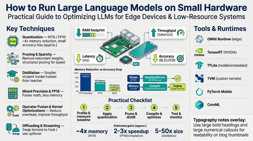
Start by inventorying the platform exactly: CPU type and core count, instruction set (ARMv8, x86_64), presence of an accelerator (GPU, NPU, TPU), available RAM, swap behavior, persistent storage, and network latency. Define memory footprint (the total RAM required for model parameters, activations, and runtime heap) and working set (the subset of memory pages accessed frequently during inference), because those two drive whether a model will thrash or run smoothly. Quantization—reducing numeric precision of model weights and activations to int8 or int4—will reduce parameter size but can increase compute variability; we’ll consider its pros and cons when mapping goals to constraints. Also measure thermal throttling and power draw early; a model that performs well on a bench but triggers sustained thermal throttling won’t meet real-world SLAs.
Clarify what you’re optimizing for: is it latency for interactive chat, throughput for batch processing, energy efficiency for battery devices, or minimal cloud round-trips for privacy? Latency is the time to produce a token or a response; throughput is tokens per second across the device; accuracy is the behavioral fidelity relative to a full-precision baseline. How do you choose which to prioritize? Choose based on the user experience and operational constraints—for a conversational assistant prioritize latency and determinism, for analytics pipelines prioritize throughput and cost. Explicitly rank these priorities because every optimization (quantization, pruning, distillation, operator fusion) trades accuracy for compute or memory.
Translate constraints and priorities into hard, testable targets. Instead of vaguely saying “make it fast,” specify: maximum cold-start time, steady-state latency target (for example, 50–200 ms per token for interactive UX), maximum resident memory (e.g., keep resident set < 3 GiB on a 4 GiB device), and acceptable accuracy delta (e.g., < 5% degradation on a validated benchmark). For a real-world edge scenario—say a 4 GiB single-board computer or a mobile SoC—we might target a quantized model under 1 GiB on disk, <3 GiB peak RAM, sustained <5 W power draw, and 100 ms median latency for 32-token completions. These concrete numbers let us choose between running a smaller base model, applying 8-bit quantization, or using selective offloading to storage.
Design microbenchmarks and quality checks that validate those targets under realistic load. Measure cold-start, warm-run, and burst scenarios; profile memory with OS tools (for example, /proc/meminfo and allocator hooks) and measure CPU/GPU utilization with low-overhead profilers. Use a simple timing harness like python measure_latency.py --prompt "Hello" --tokens 128 to gather token latency and throughput, and run a small evaluation suite to compare output quality before and after quantization or pruning. Log power draw and thermal events during long runs so you can correlate latency spikes with throttling; these empirical traces are the decision data that tell you whether to prune, distill, or deploy a smaller model family.
Building on this foundation, prioritize candidate optimization paths that meet your targets rather than chasing every technique at once. With quantifiable constraints and benchmarks in hand, we can next select model families, experiment with quantization formats (int8 vs int4), and evaluate distillation or sharded execution strategies—each choice governed by the measurable goals you just defined. By converting nebulous requirements into concrete numbers, you turn model optimization for edge devices from guesswork into reproducible engineering.
Choose model and target size
Building on this foundation, the hard decision you must make next is which model family and model size will realistically meet your targets on edge devices while preserving acceptable quality. We’ll treat model size as a concrete engineering variable—parameter count, on-disk footprint, and working-set RAM—not a marketing label—and pair that with quantization and distillation strategies you can deploy. How do you pick the right model size for your device and SLA? Start by converting your earlier constraints (RAM, power, latency) into an explicit maximum parameter budget and an accuracy budget we can measure.
The first practical step is mapping parameter counts into categories you can reason about during trade-off planning. For planning purposes, call models with <100M parameters tiny, 100M–1B small, 1B–7B medium, and >7B large; these ranges guide expectations for latency, throughput, and memory. Choose a model family that matches your task profile (causal/decoder-only models for chat and generation; encoder-decoder for translation/QA) and then pick the parameter tier that fits the resident memory you measured earlier. This approach prevents the common mistake of attempting a 30B model on a 4 GiB device and then guessing which optimization will save it.
Quantify memory and compute before you run experiments: estimate parameter bytes, runtime activation overhead, and workspace memory for operators. A small helper you can drop into your toolkit is a straightforward estimate function; for example:
# rough memory estimator (bytes)
def estimate_memory(params, dtype_bytes=4, activation_factor=1.3):
    param_mem = params * dtype_bytes
    activation_mem = param_mem * activation_factor
    overhead = 100 * 1024 * 1024  # reserve ~100MiB for runtime/heap
    return param_mem + activation_mem + overhead

# Example: 3e9 params, float32
print(estimate_memory(3_000_000_000, dtype_bytes=4)/1024**3, "GiB")
Use this to compare float32, float16, int8, and int4 scenarios: changing dtype_bytes from 4 to 2 to 1 to 0.5 approximates float32→float16→int8→int4 (accounting for packing inefficiencies). This arithmetic tells you whether pure quantization can get a model under your RAM cap, or whether you must also distill or shard.
When pure quantization isn’t enough, choose between distillation, pruning, or switching to a smaller architecture. Distillation reduces model size by training a smaller student to mimic a larger teacher; it’s most valuable when you need behavioral fidelity close to a larger baseline with lower latency. Quantization reduces memory and often increases throughput but can introduce accuracy drift; use mixed-precision (activations float16, weights int8) when you need a balance. If latency is your primary SLA, prioritize a distilled 1–3B model with aggressive int8/int4 quantization; if throughput and batch efficiency matter, prefer a larger quantized model on a device with a capable accelerator.
Apply simple decision heuristics to accelerate iteration: if your estimated memory with int8 is under the device RAM cap and latency targets look achievable from microbenchmarks, proceed with quantization-first. If int4 gets you below the threshold but introduces quality regressions, try targeted distillation to recover behavior. Ask yourself: “When should I distill versus quantize further?” Distill when you need quality back without increasing latency; quantize further when memory is the binding constraint and some accuracy loss is acceptable.
Finally, treat model selection as an iterative mapping from constraints to a concrete artifact: pick a family and parameter tier, run the memory estimator and a small latency harness, then apply quantization or distillation based on the gap to your targets. We’ll next evaluate quantization formats and sharded execution strategies with concrete microbenchmarks, but for now ensure your chosen model size is something you can repeatedly measure, tune, and deploy on your target edge devices without surprise thermal or memory failures.
Use 8-bit and 4-bit quantization
Building on this foundation, aggressive quantization is the single most effective lever to get large models running on constrained hardware like edge devices while keeping acceptable quality. Quantization reduces the per-parameter memory footprint and can unlock optimized integer kernels on CPU and accelerator hardware, but it also forces you to confront distributional shifts in weights and activations—how do you balance memory savings against accuracy loss? We’ll walk through practical patterns for int8 and int4 workflows you can apply immediately and how to validate them against the targets you defined earlier.
The core idea is straightforward: represent weights with lower bit-width numeric formats so the model consumes fewer bytes and moves less data during inference. With int8 you typically halve the memory compared to float16 and leverage many mature int8 GEMM kernels; int4 halves the int8 size again but increases sensitivity to outliers and quantization error. Quantization is not a single toggle—choices like per-channel versus per-tensor scaling, symmetric versus asymmetric ranges, and how you handle activation ranges materially affect final quality, so treat these as knobs rather than binary options.
For production-grade results, use per-channel scaling for linear layers and bias-corrected quantizers where possible. Per-channel quantization lets each output channel (or row of a weight matrix) keep its own scale factor, which preserves dynamic range for layers with heterogeneous weight magnitudes; for attention and feed-forward blocks this matters a lot. If you are doing post-training quantization (PTQ), run calibration over a representative prompt corpus to capture activation ranges; if quality degrades too much, fall back to quantization-aware training (QAT) on a distilled or task-specific dataset to recover behavior.
Apply mixed-precision strategies to get the best trade-offs: keep activations in float16 (or even float32 for critical layers) while quantizing weights to int8, and reserve int4 for models where memory is the binding constraint and you can accept additional engineering to maintain fidelity. Int8-first is the pragmatic path for interactive applications because it preserves most of the model’s behavior while materially reducing RAM and enabling faster integer math. Use int4 selectively: quantize only some layers (for instance, large MLPs or the KV cache) or use block-wise reconstruction techniques to limit error accumulation; when you need to shrink a 7B model into a device with tight RAM, that targeted int4 approach often wins over blanket quantization.
A compact calibration pattern you can drop into your pipeline looks like this (pseudo-Python):
# gather activation ranges across calibration prompts
mins, maxs = {}, {}
for prompt in calibration_prompts:
    act = run_forward_until_layer(model, prompt, layer)
    mins[layer] = min(mins.get(layer, inf), act.min())
    maxs[layer] = max(maxs.get(layer, -inf), act.max())
# compute scale and zero_point for per-channel quant
scale = (maxs - mins) / (qmax - qmin)
quantized = round(weights / scale)
Use those per-channel scales to build your quantized weight tensors, and verify with a small held-out evaluation set that perplexity or task metrics remain within your acceptable delta. Measure not only mean accuracy but also tail behaviors—hallucinations and prompt-specific regressions are common failure modes after quantization and must be detected by targeted tests.
When you deploy, prefer runtimes and kernels that are optimized for the chosen bit-width and hardware. Integer-packed GEMM performance depends on packing layout, alignment, and whether the CPU/GPU supports efficient int8/int4 arithmetic; on many mobile NPUs you’ll get much larger wins by aligning to the vendor’s preferred block sizes. Finally, tie quantization decisions back to your benchmarks: if quantizing to int4 breaks a latency or quality SLA, step back to int8 or combine quantization with a small distilled model or sharded execution to meet your constraints.
Taking this approach—calibrated PTQ, selective int4 application, and mixed-precision fallbacks—lets you move from estimates to reproducible deployments on constrained hardware. As we discussed earlier about choosing model size and measuring working set, use these quantization patterns in short iterative cycles and validate against the concrete latency, memory, and accuracy targets you established so you can confidently pick the next optimization (distillation, pruning, or sharded execution).
Prune, distill, and apply LoRA
Building on this foundation, pruning, distillation, and LoRA form the practical toolkit you’ll use when raw quantization and model selection still leave you short of your device targets. Start by treating pruning as a controlled model compression lever, distillation as a behavioral transfer method, and LoRA as a low-cost fine-tuning adapter that preserves model fidelity while shrinking the deployable footprint. These three techniques interact: the right sequence can recover accuracy lost to aggressive int8/int4 quantization or enable a smaller student model that meets strict latency and memory SLAs on edge devices. How do you decide which to run and in which order? We’ll make that decision process concrete with patterns you can reproduce.
Pruning is about removing redundant parameters while keeping the functional core intact, and you should approach it with measurement-first rigor. Begin with structured pruning (entire attention heads, MLP blocks, or channels) when you need predictable runtime gains on real hardware, and use magnitude-based unstructured pruning only if your runtime supports sparse kernels; otherwise sparsity gives you theoretical gains but no wall-clock speedup. Apply iterative, gradual pruning schedules—drop 10–20% of parameters, retrain briefly, evaluate tail-case behaviors—and track both your token-level latency and task metrics (perplexity, F1, or a domain-specific score). For example, pruning 30% of weights in a 7B model’s feed-forward layers often reduces memory and slightly lowers latency, but you must validate hallucination rates on prompts representative of your production workload.
Distillation transfers behavior from a larger teacher into a smaller student, and it’s your primary tool when you need quality close to a big model with a much smaller footprint. Use knowledge distillation with a combination of soft-target (logit) matching and task-specific loss; match teacher logits at higher temperature for softer probabilities, and mix that with ground-truth supervision to preserve task fidelity. Distillation shines when latency is the binding constraint: a distilled 3B student can deliver conversational quality near a 7B teacher while running comfortably on a mid-range SoC once quantized. When you have labeled or task-specific datasets, prioritize task-aware distillation; when you need general-purpose behavior, run data-efficient distillation using diverse prompts sampled from your expected input distribution.
LoRA (Low-Rank Adaptation) provides a complementary, lightweight approach to fine-tune or personalize models without full-weight updates, and it’s particularly useful on resource-constrained deployments. Conceptually, you replace a weight update with a low-rank decomposition W’ = W + A B where A and B are small-rank matrices; this adds a tiny number of parameters and preserves the frozen base model. In practice, apply LoRA to attention and MLP projection layers with rank r between 4 and 32 depending on the model size, and use LoRA adapters to recover accuracy lost to pruning or to encode domain-specific behavior without shipping a full model. Because LoRA stores only adapter weights, you can switch behaviors by loading different adapters on-device or in memory-constrained contexts.
Combine these tools with an experimental recipe that respects your benchmarks: first validate quantization and then decide the next step based on the remaining gap to targets. If quantized int8 meets memory but quality drifts, apply targeted pruning plus a short LoRA fine-tune to regain fidelity; if memory still binds, distill to a smaller student and then apply mixed-precision quantization with selective int4 on large MLP blocks. Iterative order matters: distill-to-size before aggressive pruning when latency is critical, prune-first when you need predictable reduction of working set; use LoRA post-prune or post-distill to tune edge-case behaviors without retraining the whole model. Always run the microbenchmarks from earlier sections—cold start, warm-run, tail-latency—after each transformation.
These approaches give you a practical pathway from a capable baseline to a deployable artifact that fits your device constraints. In the next section we’ll take those pruned, distilled, and LoRA-adapted artifacts and evaluate operator-level optimizations and sharded execution strategies so you can convert model reductions into real, repeatable latency and power wins on edge hardware.
Optimize runtime with ONNX/TensorRT
Building on this foundation, a pragmatic runtime strategy is the single most effective way to turn model-size and quantization gains into real latency and memory wins on-device. Use ONNX and TensorRT as the production bridge between a model artifact and the fastest, smallest inference engine your hardware supports. How do you pick and tune that bridge so the gains from distillation, pruning, and int8/int4 quantization actually appear in token latency and resident memory? We’ll walk through the practical pipeline and runtime knobs you’ll use in production.
Start by understanding what each piece buys you: an ONNX export gives you a hardware-agnostic graph that enables operator fusion and static analysis, while a TensorRT engine applies aggressive kernel selection, layer fusion, and platform-specific code generation to minimize runtime cost. Use ONNX for portability and early validation (dynamic axes, operator coverage), and choose TensorRT when you have an NVIDIA GPU or accelerator and need peak throughput and compact serialized engines. The right choice depends on your SLA: favor TensorRT when throughput and low-latency deterministic kernels matter; favor the ONNX stack or ONNX Runtime when you need cross-device compatibility.
The export step is where many deploys break; get it right once and subsequent builds are reproducible. Export your trained model with explicit opset and dynamic axes so batching and sequence length behave correctly. Example PyTorch export pattern:
# Export to ONNX with dynamic batch and seq dims
torch.onnx.export(model, sample_input, "model.onnx",
                  opset_version=17,
                  input_names=["input_ids"],
                  dynamic_axes={"input_ids": {0: "batch", 1: "seq"}},
                  do_constant_folding=True)
Validate the exported graph with a handful of representative prompts to catch unsupported ops and shape mismatches before you move to engine building.
When building a TensorRT engine, start with a conservative workspace and iteratively enable FP16 then INT8 with calibration. On command line, trtexec gives a fast feedback loop for microbenchmarks and engine serialization; set max workspace, enable fp16, and run calibration with a representative dataset when testing INT8. For production, use the TensorRT Python builder or ONNX Runtime with the TensorRT execution provider to programmatically control builder flags, optimization profiles, and per-layer precision fallbacks. Remember to persist the serialized engine and version it alongside its ONNX graph so you can reproduce a failing behavior without re-building on-device.
At runtime, integrate engines in a way that minimizes copies and startup cost. Load serialized engines with memory-mapped IO where possible, bind inputs/outputs once and reuse CUDA streams to overlap compute with pre/post-processing, and prefer fixed optimization profiles for common batch/sequence pairs to avoid runtime recompilation. Profile with low-overhead tracing (for example, CUDA profiling tools) to detect memory peaks and throttling; these traces often reveal that the KV cache or a large MLP block dominates resident memory and must be targeted with selective int4 or offloading.
Finally, tie runtime engineering back to your targets and benchmarks. Measure cold-start, warm-run latency, and tail-percentile latency with the same harness you used for earlier microbenchmarks, then iterate: enable fp16 for immediate throughput gains, enable int8 with calibration to reduce memory and bandwidth, and rebuild engines when you change the model or quantization scheme. Taking this approach turns ONNX and TensorRT from black-box accelerators into predictable levers you can dial to meet latency, memory, and energy SLAs on constrained hardware, and prepares you to evaluate operator-level fusions and sharded execution strategies next.
Memory mapping and offload strategies
Building on this foundation, the single biggest lever to fit larger models into tight RAM budgets is strategic memory mapping and targeted offload of cold or bulky state. Memory mapping lets you map serialized weight blobs or runtime artifacts into your process address space without immediately materializing their pages, and offload strategies push rarely accessed tensors (or the KV cache) out to slower storage so the device resident set stays within your target. When should you mmap versus eagerly load, and what should you offload first to avoid disastrous tail-latency page faults? Answering those questions with concrete heuristics prevents surprises when you move from lab benchmarks to real users.
Use memory mapping (mmap) to reduce cold-start peaks and to defer page population until data is actually used. By mapping weight files read-only into virtual memory, you avoid allocating large contiguous heaps at startup and let the OS serve pages on demand; this keeps your resident memory (RSS) aligned with the working set rather than the full model size. Practical implementations combine compressed on-disk layouts with mmap so you can transparently map quantized weight shards; when a layer is first touched the kernel faults in the needed pages, which you can monitor and correlate to layer-level access patterns.
Offload decisions should be driven by access frequency and latency sensitivity: keep the attention projection matrices and the most-reused MLP sub-blocks resident, and offload large, infrequently-read tensors such as checkpointed optimizer state, rare-attention caches, or cold model shards. The KV cache is a canonical candidate for offloading because its lifetime and access pattern are predictable—older tokens are read far less often than recent ones—so you can implement a tiered cache where hot KV pages live in RAM and older pages spill to NVMe or host memory. Offloading is not free: every tier hop adds latency and power cost, so treat offload as a trade-off between peak RSS and acceptable token latency.
Implement offload with asynchronous I/O, prefetching, and double-buffering to hide storage latency. A common pattern is to serve the immediate working set from RAM while a background IO thread prefetches the next block of KV pages or weight shards the runtime predicts you will need; when the forward pass reaches a prefetched page you get a memory-local read instead of a blocking page fault. The pseudo-pattern below illustrates a minimal async prefetch loop:
# pseudo-code: async prefetch for KV cache pages
while running:
    next_pages = predict_pages_for_next_tokens(prompt_history)
    for p in next_pages:
        if not resident(p):
            io_worker.prefetch(p)
    process_next_token()
This pattern reduces tail latency at the cost of a small background CPU and IO footprint—measure and tune the prefetch horizon against your device’s I/O bandwidth. On flash-backed storage prefer larger sequential reads and align to the vendor’s block size; on network-backed swap prefer batching to amortize latency. Monitor page-fault rate, percentiles of token latency, and power/thermal metrics to decide whether to increase prefetch aggressiveness or to move more of the working set permanently into RAM.
Combine offload with quantization and operator-level choices to maximize wins. For example, keep critical layers quantized to int8 and resident, while storing rarely used large MLP weight shards in int4 on disk and memory-mapping them; when accessed, decompress or repack them into a small in-RAM working buffer. If you’re using ONNX/TensorRT, memory-map serialized engines where supported and load-binding pointers for resident subgraphs; this reduces startup and gives you precise control over which subgraphs are resident versus pageable.
Finally, treat mapping and offload strategies as part of your continuous benchmark loop rather than a one-time hack. Profile cold-start and tail-latency with realistic prompts, iterate on which tensors you pin in RAM, and use those traces to inform pruning or distillation if offload costs are too high. Taking this measured approach to memory mapping and offloading turns constrained devices into dependable inferencing platforms rather than fragile experiments, and prepares you to apply the next layer of runtime and sharded execution optimizations.
