RNNs vs Transformers Overview
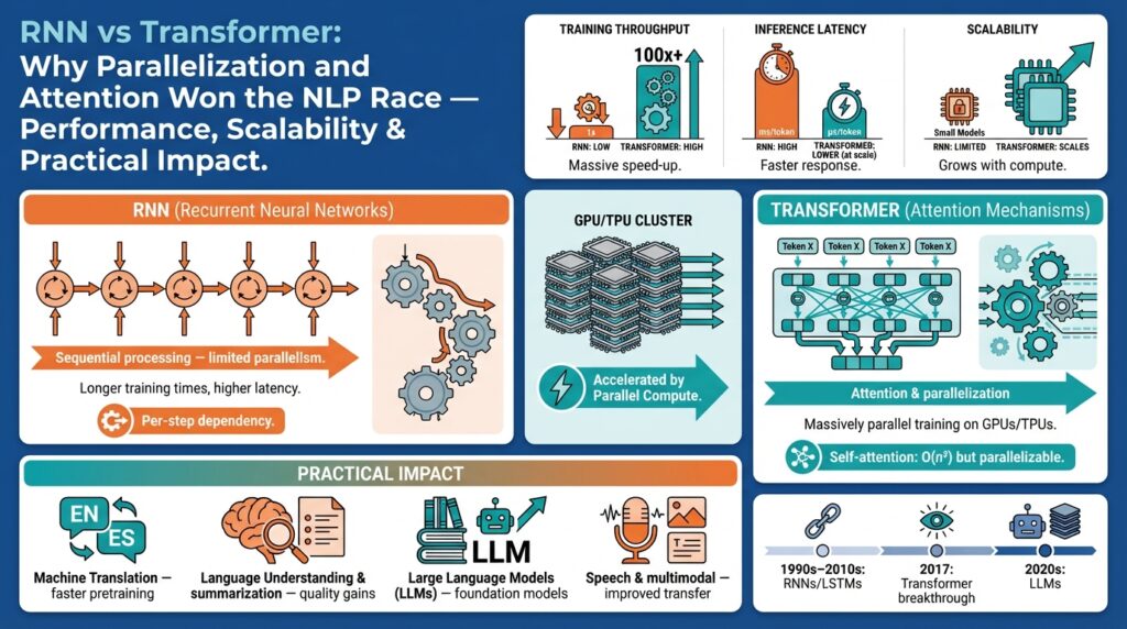
The shift from recurrent models to attention-first architectures reshaped how we build NLP systems because parallelization and global context changed what’s feasible in training and inference. In practice, you’ll see this as orders-of-magnitude differences in throughput on modern accelerators and markedly better handling of long-range dependencies. Right away, key terms matter: RNN (recurrent neural network) denotes models that process sequences step-by-step, while Transformer refers to architectures built on self-attention — a mechanism that lets every token attend to every other token. Understanding these trade-offs is essential when you choose models for production workloads or research experiments in NLP.
RNNs are stateful sequence processors that update a hidden state as tokens arrive; this sequential recurrence is their defining characteristic. Variants like LSTM (long short-term memory) and GRU (gated recurrent unit) were invented to mitigate vanishing gradients and help learn dependencies across tens or hundreds of timesteps. Because RNNs compute h_t = RNNCell(x_t, h_{t-1}) you cannot fully parallelize across time during training, which constrains batch-level throughput and makes them slower on GPUs for long sequences. Where RNNs still shine is streaming or online scenarios: when you must process token-by-token with minimal lookahead (for instance, real-time speech recognition or small-footprint edge models), the incremental state update is a meaningful advantage.
Transformers replace recurrence with self-attention, allowing each element to aggregate information from the entire sequence via attention weight matrices. Self-attention computes attention scores using matrix multiplies (Q K^T / sqrt(d)), which you can parallelize across sequence positions and across batches — this is where parallelization gives huge training speedups on GPUs/TPUs. Transformers also use positional encodings to preserve order because attention by itself is permutation-invariant. The practical effect is that transformers capture long-range dependencies more directly and at scale, which is why pretraining methods like masked language modeling and autoregressive objectives produce strong downstream performance in many NLP tasks.
Comparing performance and scalability, the crux is sequential dependency versus dense, parallelizable computation. RNNs have O(n) per-step dependence but lower per-step compute, while vanilla self-attention is O(n^2) in sequence length because of pairwise token interactions; however, the matrix-multiply nature of attention maps very efficiently to modern hardware, so end-to-end training wall-clock time is often much lower for transformers despite higher algorithmic complexity. In production, this translates to higher throughput and simpler distributed training for transformer-based models, but also higher memory pressure for very long contexts — a trade-off we must manage with sparse attention, chunking, or memory-compressed layers.
So when should you pick an RNN over a Transformer? Choose RNNs for strict streaming constraints, extremely tight memory budgets, or when you want a tiny, incrementally updated model on-device. Choose transformers when you need high-quality contextual representations, large-scale pretraining, or to exploit accelerator parallelization. For autoregressive generation, practical optimizations bridge the gap: cache keys and values during decoding so you don’t recompute attention for past tokens (e.g., append new KV pairs and compute attention against cached matrices), which recovers a lot of RNN-like incremental efficiency while keeping transformer expressivity.
Taking this forward, the reason attention-plus-parallelization dominated is not magical accuracy alone but an engineering stack effect: attention enables dense, hardware-friendly compute patterns, and parallelization unlocks feasible pretraining at scale. As we move into deployment trade-offs and scalability tactics, we’ll examine concrete benchmarks, memory-reduction techniques, and throughput-optimized decoding patterns that show how these architectural differences play out in real systems and at production scale.
Sequential vs Parallel Processing
Parallelization, attention, RNN, and Transformer are the core terms we need up front because they determine whether a model processes data sequentially or in parallel—and that choice drives performance and design decisions. When you evaluate architectures, ask: how much of the computation can run across tokens at once versus being forced to wait on prior timesteps? This question determines throughput on GPUs/TPUs, latency for streaming inputs, and the feasibility of large-batch pretraining. In the next paragraphs we’ll show concrete trade-offs and when to favor one pattern over the other.
Sequential processing is defined by a strict time dependency: each output depends on a hidden state produced by the previous token. With RNNs we update an internal state per timestep and propagate it forward, which makes per-step compute cheap but prevents parallel execution across time. That sequential dependency is an advantage for streaming or low-latency incremental systems because you can emit tokens as soon as they arrive with constant memory for the state; however, it caps achievable throughput on accelerators where parallel matrix operations are most efficient. For workloads like on-device speech recognition or very small-footprint models, the RNN’s sequential pattern often wins because it minimizes working memory and avoids recomputing context for every new token.
Parallel processing flips that model by removing the hard time-step dependency and operating on the whole sequence at once. Transformers implement this through attention, computing query, key and value matrices and using batched matrix multiplies to produce context-aware representations for every token in parallel. Because attention is expressed as dense linear algebra (Q K^T / sqrt(d)), you can fully leverage GPU/TPU parallelization and large batch sizes to dramatically lower wall-clock training time despite attention’s O(n^2) algorithmic cost. That parallelization advantage is why large-scale pretraining and high-quality contextual embeddings became feasible at internet scale: hardware utilization improves more than the raw algorithmic complexity would suggest.
The compute and memory trade-offs are explicit and actionable. Sequential RNN passes are O(n) across length with constant per-step state, making them memory-friendly for long streams; parallel attention is O(n^2) in memory for naive implementations, which creates pressure on device RAM for long contexts. Consequently, when you design systems for long documents or extremely long context windows, you must adopt mitigations such as sparse attention, windowed/chunked attention, or memory-compressed layers to reduce quadratic memory growth. These adjustments let you keep the benefits of attention’s parallelization while bounding memory use, and they often integrate nicely with distributed training strategies.
In practice you’ll also balance training throughput versus inference latency. During training, transformers shine because you can shuffle, batch, and run huge matrix multiplies that saturate accelerators; during autoregressive inference, naive transformers are sequential in generation because each new token attends to prior outputs. We recover much of the RNN-like incremental efficiency by caching keys and values and appending only the new token’s contributions—this pattern reduces redundant work and makes decoder-latency acceptable for many production systems. When latency constraints are extremely tight and lookahead is impossible, an RNN or a heavily optimized causal-transformer with aggressive KV caching and quantization may be the right engineering choice.
So how do you decide in real projects? Choose a transformer when you can exploit parallelization for large-batch pretraining, need strong long-range context, and can budget device memory (or use memory-reduction techniques). Choose an RNN when you must guarantee minimal working memory, need true token-by-token streaming with minimal lookahead, or are constrained by inference compute on tiny devices. Weigh these choices against your deployment constraints—throughput, latency, memory, and maintainability—and you’ll find hybrid patterns (chunking, local attention, KV caching) that capture the best of both worlds and set up the next phase: optimizing decoding and memory-reduction strategies for production workloads.
Self-Attention Mechanism
Attention powers the leap from stepwise recurrence to fully parallel sequence modeling, and you see that most clearly in how tokens exchange information through queries, keys, and values. In transformer models we compute a query vector for each token, a key vector that describes how a token should be matched, and a value vector that carries the content to be aggregated; this pattern—self-attention—lets every position attend to every other position in one dense linear-algebra operation, which is why parallelization becomes the dominant performance story early in training. How do you get practical leverage from this pattern in real systems? By mapping attention to large batched matrix multiplies and then applying a few engineering patterns that preserve order and efficiency.
At the algorithmic core we use scaled dot-product attention: Q K^T / sqrt(d) followed by a softmax to produce attention weights that multiply V. Here Q (queries), K (keys), and V (values) are linear projections of the token embeddings, and the scale 1/sqrt(d) keeps gradients numerically stable as dimensionality grows. In code terms (PyTorch-style) you typically implement this as three linear layers, a batched matmul for scores, a mask for causal/sequence constraints, softmax, and a final matmul with V; this pipeline is all matrix operations, so hardware-friendly and straightforward to parallelize across sequence positions and batches.
Multi-head attention extends this by projecting Q, K, V multiple times and concatenating the per-head outputs, which gives you parallel subspaces that learn different relational patterns (syntactic, semantic, positional cues, etc.). That structure helps capture long-range dependencies that RNNs struggle with because information can flow between distant tokens in a single layer instead of being propagated step-by-step. In practice you’ll see this as better gradient propagation for long contexts and more direct modeling of pairwise interactions, which is why pretraining objectives that exploit millions of tokens benefit strongly from attention-based architectures.
The trade-offs are concrete: naive attention is O(n^2) in memory and compute with respect to sequence length because you materialize an n-by-n score matrix, so for very long documents you must adopt mitigations like local windowing, sparse patterns, low-rank factorization, or chunked attention to keep memory and latency in check. For autoregressive inference we recover much of RNN-like efficiency by caching and appending key/value tensors for past tokens so the model only computes attention for the new query against cached K/V—this reduces redundant work when you generate tokens sequentially. When you implement these mitigations, pay attention to alignment between chunking and positional encoding, numeric precision (fp16/ bf16), and operator fusion to avoid extra memory copies that negate the gains of parallelization.
When you integrate attention into a production pipeline, focus on three practical items we use daily: efficient Q/K/V projection (fused kernels where possible), careful masking for causal or padded sequences, and KV caching for low-latency generation. A minimal PyTorch pattern looks like: q = Wq(x); k = Wk(x); v = Wv(x); scores = (q @ k.transpose(-2,-1)) / sqrt(dk); weights = softmax(scores + mask); out = weights @ v—this expresses the whole operation as batched matmuls so you can profile and optimize the hot path. Building on this foundation, the next section will examine decoding strategies and memory-reduction techniques that let you deploy transformer models at scale without blowing your memory budget.
Training Speed and Efficiency
If your pretraining jobs feel interminable or your dev cluster sits underutilized, the culprit is usually a mismatch between algorithmic structure and hardware leverage. Transformers leverage attention and large batched matrix multiplies to translate algorithmic complexity into high accelerator utilization, which directly improves training speed and efficiency on GPUs and TPUs. In contrast, RNNs’ timestep-by-timestep dependence limits how much work you can batch across the time dimension, so even with lower per-step compute they often yield lower throughput on modern accelerators. Understanding how to map model structure to hardware is the first practical step toward faster, cheaper training.
Building on this foundation, the most impactful levers you can pull are those that increase arithmetic intensity and reduce memory stalls. Increase global batch size and use gradient accumulation to amortize kernel launch and I/O overhead; enable mixed precision (fp16 or bf16) so tensor cores carry more work per cycle; and prefer fused kernels for Q/K/V projections and softmax where available. These techniques let attention’s dense linear algebra dominate runtime rather than memory copies or small kernels, which is why parallelization and attention produce superior wall-clock training even when attention is O(n^2) in theory.
How do you practically combine these levers? Start with a minimal PyTorch pattern: wrap forward/backward in torch.cuda.amp.autocast for mixed precision, accumulate gradients for N micro-batches to simulate a larger batch, and call optimizer.step() only after accumulation completes. Example:
scaler = torch.cuda.amp.GradScaler()
accum_steps = 8
for i, batch in enumerate(dataloader):
    with torch.cuda.amp.autocast():
        loss = model(batch) / accum_steps
    scaler.scale(loss).backward()
    if (i + 1) % accum_steps == 0:
        scaler.step(optimizer); scaler.update(); optimizer.zero_grad()
This pattern preserves your effective batch size without requiring a single host to hold all micro-batches in memory. Combine it with careful learning-rate scaling (linear scaling or warmup schedules) and you’ll retain convergence while improving throughput. Also prioritize I/O and preprocessing: asynchronous data loading, prefetch to GPU, and batching by sequence length (bucketing) to avoid excess padding.
When you need to scale beyond a single device, pick the right parallelism strategy: data parallelism (with sharded optimizers like ZeRO) minimizes implementation complexity and scales well for large batch pretraining, while tensor/model parallelism and pipeline parallelism let you spread a single huge transformer across devices. Use activation checkpointing to trade extra compute for lower peak memory when model activations dominate, and enable optimizer state sharding to sidestep memory blow-up from Adam/AdamW states. These techniques preserve training speed by keeping GPUs fed with work instead of idle waiting on memory transfers.
Profiling gives direction: measure steps/sec, GPU utilization, SM throughput, and PCIe/NVLink transfer rates to decide whether you’re compute-bound, memory-bound, or bandwidth-bound. Tools like NVIDIA Nsight Systems, nvidia-smi, and framework profilers surface hot kernels and memory spikes so you can target fixes—maybe you need fused attention kernels, maybe you need larger micro-batches, or maybe your dataloader is the bottleneck. Ask: are GPUs at 90% utilization with low host-to-device bandwidth? Then optimize kernels and computation. Are GPUs under 50% with high memory pressure? Then apply sharding and checkpointing.
Ultimately, training speed and efficiency are an engineering composition problem: architecture (attention vs recurrence), numerical strategy (mixed precision), batching strategy (global batch + accumulation), memory management (checkpointing, sharding), and I/O must all align. For most large-scale NLP projects you’ll choose a Transformer because attention maps well to parallel hardware, then apply the memory and distributed strategies above to control costs and latency. Taking these steps prepares you for the next optimizations—decoding patterns and memory-reduction techniques—that extract the final percent improvements needed for production-scale deployment.
Scalability and Resource Tradeoffs
Building on this foundation, the practical trade-offs you face are less about raw accuracy and more about throughput, latency, and resource budgets. Transformer and attention-based models give you enormous parallelization and scalability for pretraining and batch inference, but that advantage comes with a price: quadratic memory behavior as sequence length grows. How do you decide when to accept higher peak memory for much faster wall-clock training, or when to favor a smaller, sequential RNN that keeps a constant working set? Framing the decision in those operational terms lets us choose optimizations deliberately rather than by intuition alone.
From an algorithmic and hardware perspective, the core trade-off is clear: RNNs have O(n) time and constant per-step state, while naive self-attention in a Transformer produces an n×n score matrix and thus O(n^2) memory and compute with respect to sequence length. In practice this matters because attention matrices are dense tensors you must materialize or stream, and their size scales quadratically in tokens — with fp16/bf16 you still pay in device RAM as contexts lengthen. Therefore, when your workload involves long documents or million-token corpora, memory becomes the gating factor for scalability even if parallelization yields faster step throughput on GPUs or TPUs.
When memory is the limiter, apply structural and algorithmic mitigations that preserve attention’s representational power while bounding resource use. Use local/windowed attention or block-sparse patterns to reduce the effective neighborhood to O(n·w) instead of O(n^2); apply low-rank factorization or Nyström-style approximations when global interactions are smooth; and consider memory-compressed attention or routing layers for extremely long contexts. Reversible layers and activation checkpointing trade extra compute for lower activation memory, which is often the most practical lever when optimizer state is constrained. Choose the mitigation aligned to the task: windowing for locality-heavy tasks, low-rank for smooth global context, and checkpointing when compute is cheaper than extra GPUs.
At cluster scale, system-level trade-offs dominate. Mixed precision (fp16/bf16) and gradient accumulation amplify arithmetic intensity to exploit parallelization; sharded optimizer strategies like ZeRO reduce per-GPU memory by distributing optimizer state at the cost of increased network communication. Tensor and pipeline parallelism let you shard very large Transformer parameters across devices but add synchronization complexity and sometimes higher end-to-end latency. Weigh these choices by asking whether you’re memory-bound, compute-bound, or bandwidth-bound: if optimizer states blow RAM, shard them; if small kernels dominate, increase batch size and enable fused kernels to improve utilization.
Inference introduces another set of trade-offs where latency and per-request cost matter more than peak throughput. For autoregressive generation, KV caching recovers much incremental efficiency: you cache past keys and values and compute attention for the new query against cached K/V rather than recomputing the whole n×n matmul. Quantization (INT8/4-bit) and distillation reduce model size and memory pressure with modest quality loss, while pruning or structured sparsity can cut runtime but often complicate accelerator utilization. In contrast, an RNN still wins when you must guarantee sub-10ms token latency with no lookahead and tiny RAM — in those streaming cases the constant-state, token-by-token pattern remains attractive.
Make decisions by measuring the metrics that matter: tokens-per-second and steps/sec for throughput, p50/p99 for latency, and peak memory (activations + optimizer + parameters) under realistic batches and sequence lengths. Profile operator hotspots and memory peaks before adding complexity — often a single fused attention kernel or enabling bf16 yields the largest win. Prioritize optimizations in this order: get mixed precision and batching right, apply KV caching and fused kernels for inference, and use sharding/checkpointing when memory still blocks scale. Taking these measurements and targeted mitigations together prepares you to implement decoding and memory-reduction techniques that squeeze production costs without sacrificing the model quality we expect from attention-first architectures.
Practical Impact and Adoption
Transformer architectures, attention mechanisms, and aggressive parallelization changed the economics of building NLP systems—fast. When you compare wall-clock pretraining and inference throughput today, transformers consistently outpace RNN-based alternatives because attention maps naturally to large batched matrix multiplies on GPUs/TPUs, letting you scale both model size and dataset size without linear increases in training time. This shift isn’t just academic; it drives vendor tooling, cloud pricing models, and the default architectures teams choose for new NLP projects. How do you evaluate whether that default applies to your workload?
Adoption in production follows a practical, measurable path: choose a transformer when throughput, contextual quality, and scale matter most. Organizations that migrated to transformers saw dramatic reductions in steps-per-epoch and improved downstream performance for retrieval, summarization, and conversational agents, because attention provides global context in each pass rather than propagating it sequentially as in an RNN. That global context plus parallelization enables large-batch pretraining strategies (mixed precision, gradient accumulation) that substantially cut time-to-quality and make transfer learning practical for many teams.
Real-world use cases make the impact concrete: search ranking pipelines replaced RNN encoders with transformer embeddings to capture long-range signals across documents; customer-support bots moved from LSTM intent classifiers to fine-tuned transformer encoders for richer context and fewer edge-case failures. In low-latency generation services, teams combined autoregressive transformers with KV caching and sharded serving to achieve acceptable p50/p99 latency while keeping throughput high. These changes are operational — they affect hardware procurement, CI/CD, monitoring, and SLOs — not just model accuracy numbers.
Operational trade-offs are the core engineering questions you’ll face. During inference you must balance model latency and per-request cost: KV caching (store keys/values per layer and append new ones at each step), operator fusion, and quantization are the primary levers to reduce compute without losing much fidelity. How do you choose among them? Measure tokens-per-second, memory footprints, and tail latency under realistic request patterns; those metrics tell you whether to prioritize aggressive quantization, distillation, or a leaner RNN-style streamable model.
There remain situations where an RNN still makes sense: streaming audio transcription, tiny on-device models, or systems with strict constant-memory constraints. In those cases, the RNN’s incremental state update gives predictable memory behavior and minimal working set, which is valuable when you cannot afford KV caches or sharded serving. In contrast, when you need large-context reasoning, few-shot capabilities, or to exploit cluster-level parallelization, transformers and attention win because they let you amortize compute across tokens and across many accelerators.
If you’re planning a migration, take a staged approach: prototype with a smaller transformer on your representative data, profile GPU/TPU utilization and memory, then enable mixed precision (bf16/fp16) and fused attention kernels to maximize throughput. Instrument for p50/p99 latency, peak memory (activations + optimizer + parameters), and network bandwidth if you plan to shard optimizer state; these measurements guide whether you add ZeRO-style sharding, activation checkpointing, or local-window attention to control memory growth.
Adoption also shifts organizational practices: SRE and ML-engineering teams must support larger model artifacts, sophisticated caching layers, and more complex deployment topologies. We see tooling investments—model registries, KV-cache-aware serving, and observability for attention-heavy hotspots—become first-class concerns. Hiring profiles tilt toward engineers who can reason about distributed training, mixed precision numerical stability, and operator-level performance tuning rather than only sequence-modeling theory.
Taken together, the practical impact is clear: attention-first models changed how we provision hardware, measure performance, and prioritize optimizations. You should adopt transformers when your product needs large-context understanding, high throughput, and the ability to leverage accelerator parallelization; consider an RNN when streaming predictability and minimal memory are non-negotiable. Building on this foundation, the next practical stage is implementing decoding and memory-reduction techniques that squeeze costs and meet latency SLOs for production workloads.