Key Tools and Software
Building on this foundation, we immediately need a practical stack that supports rigorous data science, robust statistical methods, and reproducible economic analysis from exploration to deployment. Start by asking a concrete question: How do you choose between Python and R for causal inference in economic analysis? Your answer depends on the ecosystem you need—Python for scalable pipelines and interoperability with machine learning, R for expressive statistical modeling and rapid prototyping—so pick tools that minimize impedance between research and production.
For data ingestion and wrangling you’ll rely on battle-tested libraries and a reproducible project layout. Use pandas or the tidyverse for table manipulation and expressive joins (pandas.merge() / dplyr::left_join()), and keep heavy SQL pushed into the database when possible to avoid moving terabytes into memory. Combine Jupyter notebooks or R Markdown for exploratory analysis with script-based modules for production-ready ETL; that separation preserves reproducibility and makes reviews and code reuse straightforward when multiple analysts collaborate on an economic dataset.
When moving to estimation, choose tools that match the statistical methods you plan to use. For linear models, panel regressions, and clustered standard errors you can use statsmodels or linearmodels in Python and fixest or plm in R; for causal inference consider EconML or DoWhy when you need double machine learning or instrumental variable workflows. We often prototype an identification strategy in R for its concise formula syntax, then reimplement in Python when scaling to large data or integrating with a model-serving pipeline; this pattern keeps inference transparent while enabling operational scale.
Time-series and panel data require different implementations and diagnostic routines than cross-sectional work. Use statsmodels.tsa or R’s vars and forecast families for ARIMA, VAR, and state-space models, and rely on plm or panelr for fixed/random effects with unbalanced panels. For real-world policy evaluation—like measuring the macroeconomic impact of a policy change—you’ll want reproducible scripts that run unit-root tests, cointegration checks, and impulse-response simulations so every diagnostic is recorded and reviewable.
Scaling estimations and experiments means moving beyond single-node computation. For large surveys or administrative data, Spark or Dask provide distributed dataframes and parallelized map-reduce operations that make applying the same regression across thousands of strata tractable. Containerization with Docker plus orchestration (Kubernetes) lets you package dependency sets and spin up worker fleets for bootstrap or simulation tasks; use these when computational cost or run-time predictability matters for an economic model that needs frequent re-estimation.
Version control, environment management, and CI/CD are non-negotiable for reproducible results and auditability. Use Git with feature branches and pull requests for model changes, pin environments with conda or renv::snapshot() for R, and run tests that validate data schemas and key statistical metrics in your CI pipeline. For deployment, wrap models in a small API or batch job with pinned dependencies and automated retraining triggers so production estimates remain synchronized with incoming administrative or high-frequency economic data.
Communicating results requires both static figures and interactive exploration. Generate publication-quality plots with ggplot2 or Altair for static reporting, and build interactive dashboards with Shiny or Streamlit when stakeholders need to drill into cohort effects or counterfactual scenarios. Choose interactive tools when users will ask “what if” questions during meetings; choose static reports for formal audits where reproducibility and archival formats are essential.
As we continue, we’ll apply this stack to a concrete case study and walk through a reproducible workflow that implements the statistical methods discussed earlier. That case will sharpen choices between libraries, demonstrate trade-offs around scalability and inference, and show how tool decisions map directly to credible, auditable economic analysis.
Data Collection and Cleaning
Building on this foundation, the first practical priority is controlling what enters our systems: raw administrative records, surveys, and scraped datasets are often inconsistent, incomplete, and misaligned with analytical needs. Treat the initial data ingestion as an engineering problem, not a one-off research task—design ingestion connectors that capture provenance, timestamps, and source metadata so you can trace every estimate back to a row in a file or table. When you standardize schemas at ingest and combine that with lightweight data wrangling (type coercion, canonicalized categorical maps, and timezone normalization), downstream models and variance estimates become much easier to audit and reproduce.
The second critical layer is explicit schema validation and data contracts between producers and consumers. Define a machine-readable contract (column names, types, allowed ranges, nullability, and business keys) and validate at the boundary using tools or lightweight libraries; for example, assert numeric ranges and cardinality after a SELECT or pd.read_sql() call before further processing. How do you handle a breaking contract in production? Fail fast, log the offending sample, and trigger a retriggerable job that snapshots the offending partition and notifies stakeholders; this prevents silent bias in panel regressions or time-series estimation when a vendor changes coding mid-series.
Missing values and outliers deserve policy-driven decisions rather than ad-hoc fixes. Start by classifying missingness: missing completely at random, missing at random, or missing not at random—this classification informs whether to impute, model the missingness as part of the estimator, or restrict the sample. Use provenance to choose imputation methods: deterministic carry-forward for administrative timestamps, median/quantile imputation within strata for skewed income data, or multiple imputation when uncertainty from missingness should propagate into standard errors. For outliers, prefer winsorization or model-based robust estimators when the outlier mechanism is measurement error; preserve extreme values when they’re economically meaningful and document that choice in your ETL pipeline.
Record linkage and de-duplication scale poorly if you rely on pairwise comparisons; adopt blocking and deterministic keys first, then augment with fuzzy matching or probabilistic linkage for the residuals. For large datasets use Spark or Dask to build a blocking key and then run a smaller fuzzy match on the candidate pairs; this preserves performance while keeping false-match rates under control. Maintain a reconciliation table that records matched pairs, match confidence, and manual-review decisions so analysts can reproduce cohort definitions used in causal inference or difference-in-differences analyses.
Automation and continuous validation are not optional for production-grade data pipelines. Implement data quality tests in CI that assert schema stability, cardinality changes, and statistical fingerprints (means, variances, quantiles) so CI failures surface distributional drifts before models consume them. Integrate lightweight monitoring—hashes of primary keys, alerting on sudden null-rate increases, and periodic sample audits—and codify remediation playbooks. When we combine these checks with containerized jobs and reproducible environments (pinned with conda or renv::snapshot()), we ensure that a failed ingestion or wrangling step is traceable, testable, and fixable without ad-hoc analysis.
These practices link directly to the estimation and deployment choices we discussed earlier: pushing joins into the database reduces runtime memory pressure, robust schema validation reduces surprise standard-error inflation, and clear provenance lets reviewers reproduce identification strategies. As we move into modeling and diagnostics, we’ll rely on the cleaned, validated tables and the audit trails you built here so every causal claim is backed by a defensible, reproducible data lineage that supports both exploration and production re-estimation.
Exploratory Data Analysis
Building on this foundation, the first practical step is rapid, systematic inspection of your tables so you can decide which identification strategies are viable and which assumptions need formal testing. How do you quickly tell whether a variable’s distribution, missingness pattern, or temporal drift will bias a panel regression or a difference-in-differences estimate? Start with targeted data exploration and lightweight summaries that answer those upstream questions before you code models. Use EDA to triage issues that will affect inference—outliers, nonlinearity, heteroskedasticity, autocorrelation, and sample selection—so model choices are driven by diagnostics rather than intuition.
A core objective is to convert opaque rows into testable statements about the data-generating process. Begin by quantifying distributional shape (skewness, kurtosis) and tail behavior for economic quantities like income or expenditure; extreme right skew often implies a log or Box–Cox transformation to stabilize variance. Define heteroskedasticity on first use: variance of the error term conditional on covariates; detect it early because it inflates standard errors if unaddressed. For missingness, characterize mechanism (MCAR, MAR, MNAR) and quantify how imputation choices propagate uncertainty—document the chosen policy and, where feasible, run sensitivity checks using multiple imputation.
Visual diagnostics accelerate pattern recognition and communicate risk to stakeholders. Plot marginal distributions with histograms and kernel density estimates, then check normality with QQ-plots; examine pairwise relationships with scatterplots overlaid by a lowess smoother to reveal nonlinearity. For panel and time-series data, use autocorrelation and partial-autocorrelation plots, and draw event-aligned stacked timelines when policy changes create discontinuities. Here’s a compact Python example you can drop into a notebook for quick inspection:
import pandas as pd
import seaborn as sns
from statsmodels.graphics.tsaplots import plot_acf

sns.histplot(df['income'].dropna(), kde=True)
sns.scatterplot(x='t', y='outcome', data=df)
plot_acf(df.set_index('date')['residuals'].dropna())
Statistical diagnostics convert visual hunches into actionable fixes. Run variance-inflation-factor (VIF) checks to detect multicollinearity that will destabilize coefficient estimates; compute Breusch–Pagan or White tests to formalize heteroskedasticity concerns and then switch to robust or cluster-robust standard errors accordingly. For panels, execute unit-root (ADF) tests to avoid spurious regressions and check cointegration when you expect long-run relationships between series. When you have treatment assignments, examine covariate balance and propensity score overlap visually and numerically to decide whether reweighting, trimming, or stratified estimation is required.
When datasets are large or stratified, scale your inspection with reproducible aggregates rather than full-table scans. Compute stratified summary tables and temporal fingerprints—means, medians, and key quantiles—per subgroup and persist them to a canonical diagnostics table so reviewers can see how distributions changed over time. Use hashing of primary-key samples and sample-preserving downsampling to reproduce plots deterministically in notebooks and CI. For survey or administrative data with sampling weights, always visualize weighted distributions; unweighted diagnostics can mislead about population-level effects.
We should also automate the obvious checks so manual effort targets subtler pathologies. Integrate data exploration steps into pre-merge tests and CI: assert that key quantiles remain within expected ranges, that new levels in categorical variables are flagged, and that a small set of statistical fingerprints (mean, variance, null-rate) are compared against historical baselines. Persist diagnostic artifacts—plots, summary CSVs, and a lightweight JSON metadata file—into your experiment tracking or data catalog so every exploratory decision is reproducible and auditable.
Finally, treat this stage as a readiness gate before estimation: if diagnostics reveal structural breaks, non-overlap, or persistent autocorrelation, adapt your identification strategy rather than forcing a standard estimator. The next step will be formal model specification and robustness checks; armed with reproducible visualizations, statistical diagnostics, and documented transformation choices, we can move into estimation with defensible assumptions and a clear plan for sensitivity analyses.
Core Econometric Methods
Building on this foundation, the core econometric methods you actually use will determine whether a finding is credible or merely believable. We start with causal inference and estimation choices up front because the estimator encodes your identification assumptions; picking an algorithm is inseparable from stating why treated and control are comparable. Practically, that means framing the research question as an estimand (ATE, LATE, ATT) before you write an equation or a line of code so every diagnostic maps back to the causal claim. How do you choose an estimator that matches the identification strategy and data-generating process?
Ordinary least squares remains the workhorse for continuous outcomes, but its validity rests on clear assumptions: linearity, exogeneity, and correctly specified functional form. When regressors correlate with the error term—through omitted variables, measurement error, or simultaneity—OLS is biased and inconsistent; diagnosing those problems with residual plots, VIFs, and testing for heteroskedasticity guides whether you need robust standard errors, transformations, or a different estimator. We typically run specification checks early: include functional-form flexible terms (splines or polynomials) and compare OLS to robust estimators to see if coefficient signs and magnitudes shift. Those shifts tell you whether your substantive story survives modest departures from the ideal assumptions.
Instrumental variables let you recover causal effects when endogeneity is present, but the strategy requires two explicit claims: relevance and exclusion. A valid instrument must strongly predict the endogenous regressor and affect the outcome only through that channel; weak instruments create bias toward OLS and inflate variance, so check first-stage F-statistics and consider limited-information estimators if necessary. In practice we prototype IV in a notebook and then reproduce it in a scalable pipeline; a compact Python pattern using linearmodels looks like this for two-stage least squares:
from linearmodels.iv import IV2SLS
model = IV2SLS(df.outcome, df[['const','x']], df[['z']], df[['instr']]).fit()
print(model.summary)
Difference-in-differences and event-study designs are the natural choice for policy evaluation when you observe treated and untreated units over time, but implementation details matter. Simple two-way fixed effects can produce biased estimates under staggered adoption or heterogeneous treatment effects, so prefer estimators that explicitly normalize dynamic effects and report lead/lag coefficients rather than a single average treatment effect. Always graph event-study coefficients with confidence intervals and run placebo leads to detect pre-trends; if pre-trends appear, re-specify the comparison set or use alternative identification such as matching on pre-treatment trajectories. These visual and falsification checks are essential to defend a DID-style identification at review.
Panel regression techniques—within estimators, random effects, and pooled models—give you leverage when units are observed repeatedly, but they trade off identification sources. Fixed effects purge time-invariant confounders by differencing within units and are a go-to when unobserved heterogeneity is plausible; random effects can be more efficient but require exogeneity of unit effects, which the Hausman test can probe. For unbalanced panels or short T/large N designs, cluster standard errors at the unit or group level to account for serial correlation and heteroskedasticity; empirical practice shows clustered inference often changes significance more than point estimates. When you need high-dimensional fixed effects (two-way or more), use specialized implementations (fixest, lfe) to avoid material memory and runtime overhead.
Time-series and structural methods belong when dynamics and equilibrium relationships drive outcomes rather than cross-sectional variation. Unit-root tests and cointegration checks prevent spurious regressions; vector autoregression (VAR) and state-space models let you estimate impulse responses and decompose shocks, which is crucial when a policy shock propagates through multiple macro series. Choose ARIMA-style models for short-run forecasting, VARs for shock decomposition, and structural models when theory gives identifying restrictions; always validate out-of-sample and inspect residual autocorrelation. In mixed-frequency or panel-time setups, combine panel fixed effects with dynamic correction methods to keep inference honest.
Robust inference and sensitivity analysis complete the workflow: you must show that results resist reasonable modeling choices and sampling variability. Use heteroskedasticity-robust and cluster-robust standard errors, bootstrap confidence intervals for small samples, and specification-curve or leave-one-out analyses to quantify researcher degrees of freedom; run placebo outcomes and alternative control groups as falsification checks. Document every transformation and pre-register key identification steps when possible so reviewers can reproduce the pathway from raw table to causal claim. Taking these practices together prepares you to move from cleaned, auditable data into models that stakeholders and auditors can credibly interrogate.
Causal Inference Techniques
Building on this foundation, when you operationalize causal inference in economic analysis you must start by pinning down the estimand and the identification strategy before you write a line of code. Causal inference, treatment effects, and identification strategy belong in your research design as concrete objects: define whether you want an ATE, ATT, or LATE and then choose techniques that map to the data-generating process. That early clarity prevents a common failure mode where model outputs are interpreted as causal without defensible assumptions, and it frames which diagnostics and sensitivity checks you will need downstream.
Different identification problems demand different tools, and knowing when to use each is practical judgment as much as technical skill. Instrumental variables are appropriate when an unobserved confounder correlates with your key regressor but you can find a credible instrument that satisfies relevance and exclusion; regression discontinuity works when treatment assignment has a clear cutoff and the running variable is as-good-as-random near the threshold. Difference-in-differences and event-study designs exploit temporal variation across treated and control units but require parallel trends or robust alternatives when adoption is staggered. Propensity score methods and matching help when selection into treatment is based on observable covariates, and synthetic control is powerful for single-unit policy evaluation with rich pre-treatment periods.
In practice, implement these methods with patterns that prioritize transparency and reproducibility rather than opaque tuning. For IV, always report first-stage F-statistics and show the reduced form alongside the two-stage estimate; a common minimal pattern is first_stage = OLS(z ~ x + controls) followed by IV = 2SLS(y ~ x + controls, instrument=z). For DID, graph event-study coefficients with clustered standard errors and run placebo leads to detect pre-trends. When you adopt machine-learning–augmented approaches like double machine learning, treat the nuisance-model training and cross-fitting as part of the estimation pipeline so you can reproduce splits and hyperparameters in CI and audit logs.
Diagnostics and robustness are not optional; they are the evidence you present to skeptical reviewers. Test balance and propensity-score overlap visually and numerically, and trim or reweight if regions of non-overlap threaten external validity. Run falsification tests such as placebo outcomes, permutation of treatment timing, and leave-one-group-out sensitivity; for panel settings, check serial correlation with cluster-robust inference or block bootstrap where appropriate. When an instrument is used, interrogate exclusion with alternative instruments or overidentification tests where available, and report sensitivity bounds (e.g., Rosenbaum-style or partial identification) if exclusion is questionable.
Scaling these techniques into production-grade analysis ties back to the tooling we discussed earlier. Use libraries that match your chosen estimator—linearmodels or EconML for IV and DML patterns, fixest or plm for high-dimensional fixed effects, and custom implementations for synthetic control when you need tailored loss functions—and wrap estimators in testable scripts. Integrate propensity-score diagnostics and event-study plots into your CI artifacts so every review includes the same visual evidence; persist seeds, sample splits, and diagnostic tables to your experiment-tracking system. When possible, pre-register the estimand and core identification steps so changes to the pipeline are visible and defensible during peer review or audits.
Ultimately, the strength of a causal claim rests on the plausibility and testability of assumptions rather than on a single preferred algorithm. Ask yourself: What would a skeptical reviewer say is the weakest assumption here, and how can we quantify its impact? By front-loading the estimand, choosing techniques that align with the data structure, automating diagnostics, and documenting every decision, we turn causal inference from a black-box exercise into an auditable, reproducible workflow. Next we will apply one of these strategies to a concrete case study and walk through the code, diagnostics, and sensitivity checks you would include in a reproducible analysis.
Machine Learning Applications
Machine learning transforms how we extract signal from messy economic data, but the central question is practical: how do you incorporate machine learning into causal workflows for economic analysis without undermining identification? We use machine learning primarily as a flexible function approximator for prediction, representation learning, and nuisance estimation that feeds into principled econometric estimators. When you approach a policy question, front-load the estimand and identification assumptions and then decide which machine learning components augment—not replace—your identification strategy. This framing keeps causal inference and machine learning complementary rather than competing priorities.
A common role for machine learning in applied economics is nuisance estimation: learning propensity scores, conditional outcome forecasts, or density ratios that plug into orthogonal estimators. These nuisance models improve efficiency and reduce bias when trained with careful cross-fitting, but they do not substitute for checks on instrument validity or parallel trends. For heterogeneous treatment effects, machine learning excels at discovering treatment effect variation across high-dimensional covariates, enabling targeted policy recommendations and uplift modeling where average effects hide meaningful heterogeneity. Taking this concept further, double machine learning (DML) gives us a principled way to combine flexible learners for nuisance components with an orthogonalized estimator for the causal parameter.
To make this concrete, implement a reproducible cross-fitting pattern: split your sample into K folds, train nuisance learners (for example gradient-boosted trees or regularized forests) on K-1 folds, predict out-of-fold nuisance components, and then estimate the causal parameter on the remaining fold using the orthogonalized moment. The cross-fitting loop prevents overfitting from contaminating the final estimator and preserves valid asymptotic inference under standard conditions. In practice, you’ll wrap this in a pipeline that persists seeds, hyperparameters, and feature transformations so reviewers can reconstruct exactly how nuisance models were trained and how the orthogonalization was applied.
Validation and robustness require more than predictive metrics. Evaluate nuisance learners on held-out data for calibration and tail behavior, and inspect how sensitive the causal estimate is to different model families, hyperparameters, and sample splits. Use honest inference methods—sample splitting, influence-function–based standard errors, and bootstrap where appropriate—to produce confidence intervals that reflect both estimation and model uncertainty. Ask reproducible falsification questions such as placebo treatments, permutation tests of timing, and bounding exercises to quantify how violations of exclusion or overlap would change your conclusions.
Operationalizing machine learning in economic analysis means treating feature engineering, model training, and serving as engineering artifacts subject to version control, testing, and monitoring. Persist feature definitions in a feature store, version datasets with hash-based snapshots, and automate retraining triggers when covariate drift or distributional fingerprints change. For interpretability and stakeholder communication, use partial-dependence plots, SHAP-style attribution, and subgroup-level event studies so policymakers understand why a model recommends targeting one cohort over another; interpretability is often the difference between an adoptable policy tool and a black box that regulators reject.
There are practical trade-offs you must weigh when deciding how much machine learning to add. Prefer classical parametric or semi-parametric approaches when samples are small, theoretical structure yields clear functional forms, or transparency and auditability trump predictive gains. Conversely, scale up machine learning when you face high-dimensional confounders, nonlinearity, or the need to personalize interventions—provided you keep orthogonality, cross-validation, and robustness checks central to the pipeline. The right choice balances economic theory, identification plausibility, and operational constraints.
Building on our earlier discussion of tooling and reproducible pipelines, the next step is to apply these patterns to a case study: implement a double machine learning estimator on administrative wage records, show the full cross-fitting code and diagnostics, and compare treatment-effect heterogeneity using interpretable feature attributions. That worked example will demonstrate how machine learning augments causal inference in practice and what engineering controls we need to keep the analysis auditable and defensible.