Advantage-Weighted Supervised Fine-Tuning for Post-Training Generative Recommenders — Improving LLM Recommendation Quality and Scalability

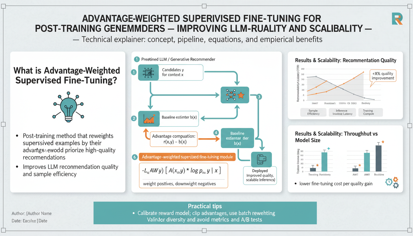
Why Advantage-Weighted Supervised Fine-Tuning (A-SFT) for Generative Recommenders? — motivation, limitations of RLHF/PPO in recommendation, and when to use A‑SFT

Generative recommenders ask a large language model to produce structured, high-quality item sequences or natural-language suggestions that directly drive user-facing metrics (CTR, watch time, conversion, NDCG). Aligning those open-ended generations to business rewards is fundamentally different from standard supervised tuning: rewards are noisy, sparse, and often derived from logged interaction data; online experimentation is expensive; and reward models can generalize poorly outside the training distribution. Advantage-weighted supervised fine-tuning (A‑SFT) is a pragmatic middle path: instead of running a full RLHF pipeline with policy optimization (PPO) or doing expensive online RL, it converts reward signals into example-level weights and trains the model with a weighted supervised objective. This preserves the simplicity and stability of SFT while recovering many of the effective policy-improvement properties of RL. Empirical work in production-scale recommender settings has shown that advantage-weighted approaches can improve recommendation metrics while avoiding several failure modes seen in direct PPO-style optimization. (netflixtechblog.medium.com)

Why the approach matters in recommendation systems: recommendation service objectives are high-volume, multi-metric, and commercially sensitive. Running full RLHF or PPO at scale requires extensive reward-labeling pipelines, careful reward-model calibration, and large amounts of online exploration to close distribution gaps. In practice this creates three major friction points: cost and labeling scale (human feedback and curated labels are expensive and slow), instability and reproducibility (policy-gradient optimizers like PPO can be finicky to tune and may diverge or oscillate), and reward-model overfitting (PPO can over-optimize the policy with respect to an imperfect reward model, producing behavior that looks good to the RM but harms real metrics). These are documented across the literature and engineering reports on RLHF and PPO, and are especially acute when the reward signal is derived from logged user interactions rather than curated human pairwise preferences. (bair.berkeley.edu)

The conceptual engine behind advantage weighting is simple and powerful. Take logged (context, model-output, reward) tuples and compute an advantage for each example: advantage = reward − baseline (the baseline can be a running mean, a value network, or a control-policy score). Turn that scalar advantage into a positive training weight (for example via a softmax-style transform like weight ∝ exp(advantage / τ) with clipping or percentile-based truncation). Then fine-tune the model using weighted maximum likelihood (minimizing −w · log pθ(output | context)). High-advantage examples pull the model distribution toward actions that empirically yielded higher reward; low-advantage examples are downweighted rather than discarded, so the model retains broad coverage and avoids catastrophic mode collapse. This weighted supervised step has strong theoretical roots in advantage-weighted regression and similar off-policy methods where supervised regressions with importance-like weights produce policy improvements while avoiding unstable gradient estimators. (arxiv.org)

Concrete implementation steps (practical recipe):

• Data and logging: collect offline interaction logs with (context, candidate sequence or completion, reward) entries. Rewards are numeric user outcomes (click, dwell time, watch, purchase) or composite business metrics. Include any available propensity/score metadata if you have it (exposure probability, logging policy id).

• Reward model and ensembles (optional but recommended): if you derive reward via a learned reward model, train an ensemble and hold out calibration sets to reduce overfitting risk. Where possible, use offline A/B or counterfactual estimates to sanity-check reward magnitudes. Netflix-style engineering work recommends ensembles/ensembling for confidence when a single RM may generalize poorly. (netflixtechblog.medium.com)

• Baseline/value estimation: compute a baseline for each context. Options include the mean reward for that context cluster, a small value network trained to predict reward, or the score of a current production policy. The baseline reduces variance and yields signed advantages.

• Advantage → weight transform: map advantage to a positive weight. The canonical choices are: softmax weighting w_i = exp(adv_i / τ), clipped or top-k truncation, or normalized weights that sum to one per mini-batch. Tune temperature τ; typical starting ranges are 0.1–2.0 depending on reward scale. Clip very large weights (e.g., top 99th percentile) to prevent a handful of high-reward outliers from dominating training. Research on importance-weighted SFT shows that these simple transforms tighten bounds to RL objectives while remaining implementation-light. (arxiv.org)

• Weighted SFT loss: train with the weighted negative log-likelihood loss L = −∑_i w_i log pθ(y_i | x_i). Include stability regularizers: a KL penalty to the starting SFT model (to avoid catastrophic policy drift), label smoothing, and dropout. Regularize the weight distribution (e.g., mix in a fraction α of uniform weighting) to keep exploration in deployed policies.

• Monitoring and safety checks: track both surrogate reward (the RM score) and offline, counterfactual/IPS-corrected business metrics if propensities are available. Use held-out human or randomized-exposure validations to detect reward-model exploitation (policy that maximizes RM but hurts real users). The Netflix engineering report specifically flags reward-model generalization and lack of IPS as key concerns — treat the RM as a noisy judge and evaluate externally. (netflixtechblog.medium.com)

• Iteration cadence: retrain and reweight periodically. If you update the reward model, recompute advantages to avoid distributional mismatch. Consider combining A‑SFT with conservative offline RL (e.g., a CQL-style constraint) if you need additional robustness in scarce-data regions (Netflix experiments noted CQL improved robustness though it sometimes underused RM signal). (netflixtechblog.medium.com)

When A‑SFT is the right tool (and when it isn’t):

• Use A‑SFT when you predominantly have logged offline signals (large-scale interaction logs), reward scalars or calibrated reward models, and a need for operational simplicity and stability. It is ideal for post-training improvement of generative recommenders where you want to tilt an existing SFT policy toward higher-value outcomes without running an expensive RL optimization loop. Production evidence suggests A‑SFT can outperform RM-heavy PPO/DPO approaches on recommendation metrics while being easier to scale and less prone to RM overfitting. (netflixtechblog.medium.com)

• Prefer full RL (PPO/RLHF or online RL) when you must explicitly explore to discover new high-value behaviors, when the decision horizon and stateful sequential credit assignment require dynamic exploration (multi-step session optimization), or when you have reliable, high-quality human preference labels tailored for alignment where reward shaping would otherwise be insufficient. PPO can be powerful in those scenarios but at the cost of complexity, compute, and careful reward-model engineering. (bair.berkeley.edu)

• Avoid A‑SFT when your logs have extreme selection bias with no propensity information and the support of better actions is missing (no coverage). In such off-policy, sparse-coverage regimes, weighted supervised learning can amplify biases; conservative offline RL or targeted online experiments may be necessary.

Common failure modes and mitigations:

• Reward-model exploitation: if the policy optimizes RM idiosyncrasies, it will appear to improve surrogate reward while harming real metrics. Mitigate via RM ensembles, held-out human validation, and conservative weight clipping. (netflixtechblog.medium.com)

• Overconcentration on a few examples: aggressive weighting without clipping causes mode collapse. Use truncation, entropy regularization, or KL penalties to the SFT prior.

• Miscalibrated advantages: poor baselines produce noisy advantages. Use simple, robust baselines (running mean per-context group) and sanity-check advantage distributions before training.

Key takeaways for engineering teams: A‑SFT converts reward signals into supervised learning leverage — preserving the scalability and reproducibility of SFT while bringing many benefits of policy optimization. It is especially attractive for large-scale recommender systems where offline logs, compute budgets, and production stability are first-class constraints. Recent academic and industrial work frames A‑SFT and related importance-weighted variants as effective RL-free or RL-lite strategies that tighten the connection between SFT and policy improvement while reducing the practical burdens of PPO-style pipelines. If your goal is to nudge a generative recommender toward business metrics with minimal rollout risk and reasonable empirical gains, implementing advantage-weighted fine-tuning with careful RM calibration, weight clipping, and robust offline evaluation is a high-leverage next step. (arxiv.org)

Prerequisites & dataset setup — logged trajectories, contextual bandit framing, cleaning/formatting sequences, and handling missing logging-policy info

Begin by designing a minimal but complete row schema for your logged interactions. Every row should record: a unique user identifier (or a privacy-preserving hash), a timestamp, canonical item (or token) identifiers for events, an event type (impression, click, view, purchase, skip, etc.), any available reward scalar (raw or precomputed — e.g., click=1, dwell>30s=1, normalized watch-time), and metadata about context (device, page layout, query, session id if present). If your system logged the model output (the full generated sequence or the recommended slate), persist that text or item-sequence as an explicit field; for generative recommenders you want both the prompt/context and the model’s completion. Store ancillary fields that help downstream debiasing and diagnostics: logging-policy id or model-version (if known), any sampling/propensity score recorded at serve time, and coarse exposure metadata (position, slot id, UI layout). Persist this as a columnar, partitionable file format (Parquet/Delta/Iceberg) partitioned by time (year/month/day) and, when practical, a coarse shard (region or bucket(user_id)) to avoid tiny files and to enable efficient date-range reads. (See recommended partitioning and file-size guidance for data-lake workloads.) (datasturdy.com)

Turn logged trajectories into training tuples. For post-training generative recommenders you will usually convert each logged event (or a small subsequence of a trajectory) into a contextual bandit example (context, action, reward, metadata). The canonical mapping is: context = user history up to time t (timestamps, item IDs, features), action = the model output or chosen item(s) at t, reward = scalar outcome observed after the action, metadata = position/slot, layout, and (if available) the logging policy’s probability for selecting that action. This one-step bandit framing is the standard offline approach for learning from logged bandit feedback: it lets you evaluate and reweight actions without requiring full environment rollouts. If your business reward is cumulative (multi-step session reward), you can either (a) attribute the terminal/trajectory reward back to earlier actions (careful — introduces credit-assignment bias), or (b) keep full trajectories and compute discounted returns per time-step — but expect greater variance and more complex baselines. Counterfactual risk minimization and IPS-based learning are the theoretical backbone for learning from such logged bandit feedback; they justify reweighting by serve probabilities when those are available. (researchgate.net)

Practical cleaning and sessionization steps (step-by-step): (1) normalize and deduplicate — canonicalize item IDs (resolve renames/A/B experiment aliases), drop duplicate event-lines, and remove server-side retries or synthetic heartbeat events; (2) bot/filter hygiene — filter known crawler user-agents and abnormal event-rate users; (3) timestamp normalization — convert all times to a single timezone/UTC, align to canonical event-time and record both event_time and ingestion_time for late-arriving events; (4) sessionize — reconstruct sessions with a configurable inactivity gap (30 minutes is a common default but tune to product behavior); use streaming/batch session windows where supported to avoid handwritten gaps-&-islands logic. Use session windows or explicit session_id when you want to convert a long trajectory into contiguous sequences. For streaming ingestion or very large datasets prefer Spark Structured Streaming or equivalent session-window primitives for stable and scalable sessionization. (Spark supports session windows natively and lets you set a dynamic inactivity gap.) After sessionization, split long sessions into fixed-length sequences (sliding windows with stride or recency-based truncation) and tag sequence boundaries so the model can learn generation boundaries. (spark.apache.org)

Sequence formatting and feature engineering checklist: (a) choose a context window length (e.g., last 50–500 tokens/items) and a truncation policy (keep most recent; optionally reservoir-sample for diversity); (b) encode item identities with a stable id → token map and an out-of-vocabulary sentinel for rare/new items; (c) include dense features (recent dwell-time, recency buckets, coarse user cohorts) and sparse context tokens (genres, categories) as structured fields or special tokens depending on model input format; (d) for generative prompts, build canonical prompt templates that concatenate event tokens, separators, and slot metadata so the model sees consistent structure; (e) create negatives: for ranking-style objectives you will need sampled negatives per context (uniform, popularity-biased, or hard negatives from a candidate generator) so evaluation metrics like NDCG/HR make sense; (f) persist prepared sequences in an ML-ready table with columns: context_text, continuation_text, reward, weight (initially 1.0), logging_policy_id, propensity (nullable), and diagnostics tags. Use bucketing (hash(user_id) mod N) if you need consistent train/validation splits without exposing user ids. For large-scale training, materialize these examples into sharded Parquet/Delta tables with deterministic sharding keys to ensure reproducible batching and easy reweighting. (datasturdy.com)

How to compute advantages and training weights (concrete recipe): choose a baseline estimator per context to get signed advantages. Simple and robust options are per-context running means (e.g., mean reward for the same user-cohort and UI layout), or a learned value network trained to predict reward from the same context features. Compute advantage_i = reward_i − baseline(context_i). Map advantages to positive weights with a soft exponential transform, then clip or truncate extremes: w_i ∝ exp(advantage_i / τ); normalize per minibatch or by dataset so weights don’t collapse training, and cap extreme weights (e.g., clip to 99th percentile or set a max multiplier). In practice a small temperature τ (0.1–2.0) concentrates learning on higher-advantage examples; tune τ on held-out offline metrics. Use a mixed objective that interpolates the weighted negative log-likelihood with a KL or MLE regularizer to the original SFT policy (mix fraction α of uniform weight) so the model keeps coverage on lower-weighted actions. This advantage-weighting idea has strong roots in advantage-weighted regression / AWR and is the practical core of advantage-weighted SFT workflows. (xbpeng.github.io)

When your logs lack logging-policy probabilities (propensities): don’t panic — there are several defensible strategies and diagnostic steps. First, recognize the risk: naive IPS reweighting with poor propensities produces high-variance or biased estimates; in addition, unobserved confounders can make propensity estimation non-identifiable. Practical mitigations: (1) use advantage-weighted SFT, which explicitly avoids reweighting by logging probabilities and instead uses advantage-derived weights from rewards/baselines — this is especially appropriate when logging-policy info is missing or unreliable. (2) if you prefer IPS-style debiasing, estimate propensities from logs by training a separate propensity model that predicts logging-action probabilities from observed context and available serve-time features (attribute-based propensity models are a pragmatic approach used in industry). (3) apply variance-reduction estimators: self-normalized IPS (SNIPS) or variance-regularized counterfactual risk minimization techniques reduce sensitivity to very large propensity ratios; and (4) use doubly-robust or DR-type estimators that combine a reward model with IPS to get lower bias/variance tradeoffs — these can improve robustness even when propensities are noisy. Important diagnostics: plot propensity histograms, compute effective sample size ESS = (sum w)^2 / sum(w^2) (where w are your importance weights), and check for lack of support (many near-zero propensities) — that indicates unreliable off-policy overlap and suggests you should reduce IPS reliance or run small randomized exposures. Several academic and production studies document these pitfalls and practical estimators and diagnostics for propensity-based learning. (netflixtechblog.medium.com)

If you must estimate propensities, follow these pragmatic steps: collect feature columns that were available at serve time (UI layout, position, query text, device, time-of-day), train a probabilistic classifier that predicts which action (or item) was served given the context, and calibrate predicted probabilities using temperature scaling or isotonic regression on a holdout. Avoid using post-hoc downstream features that leaked outcome information. When propensities are learned rather than logged, treat them as noisy measurements: use clipped importance weights, self-normalization, and incorporate variance penalization in your offline learning objective (counterfactual risk minimization). Where possible, pick a small, safe randomized experiment to validate propensity estimates and to get unbiased anchor points for calibration. Google’s attribute-based propensity estimation and other production case studies show this is feasible across many implicit-feedback scenarios when you can reconstruct the serve-time feature set. (research.google)

When to prefer a propensity-free route: if you lack serve-time logging, have serious unobserved confounding, or the estimated propensities concentrate near zero (very little overlap), prefer A-SFT / advantage-weighted supervised fine-tuning or conservative offline RL algorithms. The Netflix A-SFT workflow explicitly targets these settings: it uses advantage weighting on observed examples (no IPS) coupled with regularizers to the behavior policy to avoid runaway drift toward reward-model idiosyncrasies. If you do use such propensity-free methods, invest heavily in external validation (small randomized holds or human-labeled checks) because surrogate reward models can be exploited by the fine-tuned policy. (netflixtechblog.medium.com)

Sanity checks, monitoring, and evaluation before training: (1) inspect reward distributions across important slices (user cohorts, UI layout, item categories) and check baseline stability; (2) visualize advantage distribution and weight histogram — if a handful of examples carry most of the mass, increase clipping or lower τ; (3) compute ESS for your target policy and for IPS-weighted estimators so you understand effective sample counts; (4) run small counterfactual evaluations with SNIPS/DR estimators and compare to a held-out randomized-exposure A/B (if available); (5) run human or curator audits of high-weight examples to ensure they are genuine signals (not bot artifacts or reward-model hallucinations); and (6) maintain provenance: always keep raw logs, the preprocessed examples, and the exact code/parameters that produced advantage weights so results are reproducible and auditable. The combination of these checks will expose exploitation risks, distributional gaps, and propensity pitfalls before you deploy a model trained using advantage-weighted or propensity-weighted objectives. (researchgate.net)

A concise example transformation pipeline (pseudocode):

-- 1) raw ingestion -> canonicalized table
CREATE TABLE events_raw_parquet AS SELECT
  user_hash,
  to_utc(event_ts) as event_time,
  canonical_item_id(item_id) as item_id,
  event_type,
  ui_layout,
  serve_model_version,
  reported_propensity /* nullable */
FROM raw_event_stream;

-- 2) sessionize (batch with session gap = 30m)
SELECT
  user_hash,
  session_window(event_time, '30 minutes') as session_id,
  collect_list(struct(event_time,item_id,event_type,ui_layout,reported_propensity)) as events
FROM events_raw_parquet
GROUP BY user_hash, session_window(event_time, '30 minutes');

-- 3) explode session -> bandit examples (context = events before t)
-- produce columns: context_tokens, action_item, reward, reported_propensity

Persist the resulting examples table and then compute baseline/advantage and final weight column offline (store weights so training is reproducible). In your training loop, read the examples table, optionally filter by weight thresholds or max-example-age, and feed (context, continuation, weight) to the weighted SFT objective L = −∑ w_i log pθ(y_i|x_i) + λ KL(pθ || p0). Keep weight clipping and a small fraction of uniform-weight samples every batch to maintain coverage. (Do not forget to reserve a time-based holdout for final offline policy selection and to run external validation.) (studylib.net)

Finally, document and version every dataset artifact: raw logs, canonicalized events, sessionized sequences, computed baselines, computed advantages, weight parameters (τ, clipping percentiles), and the code that computed propensities (if any). This traceability is critical for diagnosing regressions, replaying experiments, and satisfying compliance/privacy requirements. Where required, apply privacy-preserving transforms (hashing, PII removal, differential-privacy-aware aggregation) before sharing datasets across teams. Following these steps — careful logging schema, robust sessionization and cleaning, defensible handling of missing logging-policy information, and conservative advantage-weight computation — gives you a practical, auditable dataset foundation for Advantage-Weighted Supervised Fine-Tuning and other offline policy-improvement methods. (datasturdy.com)

Building and reliable reward models for recommendation — labels, proxy rewards, calibration, and validation strategies

A robust, trustworthy reward pipeline is foundational for advantage-weighted fine-tuning in recommendation. Start by defining what you will call “reward” in explicit terms: pick a primary business signal (click, completed watch, purchase, session dwell) and decide whether you need a composite objective (e.g., 0.6watch_time_norm + 0.4conversion). For each candidate scalar, record the exact extraction rule used (SQL / event proto) and a short justification for why it correlates with the business outcome you care about. When you can, prefer signals that are both interpretable and minimally confounded (for example: explicit ratings or post-session surveys are cleaner than raw session duration when timeouts and autoplay are common). Use a reproducible unit (per-impression, per-session, per-sequence) and normalize units so reward magnitudes are comparable across slices (per-user z‑score or percentile-normalization are common). Empirically inspect reward distributions across cohorts and UI variants to detect obvious sampling bias or instrumentation bugs before you train a reward model. (netflixtechblog.medium.com)

If direct human labels are available for some proportion of the distribution, build the reward model around them as an anchor: label artifacts should be treated as gold-standard and preserved for validation and calibration. For large-scale implicit feedback, create proxy labels with documented heuristics: e.g., treat “watch > 30s” as positive for short-form, but also provide alternate labels (watch > 2m, finished_episode boolean) to allow sensitivity analysis. When using proxy labels, maintain a labeled validation slice with human judgments or randomized-exposure data so you can quantify how well the proxy matches human preference or true business lift. Hold out a small but representative stratified sample of user contexts for human labeling (budget permitting) and prioritize labeling examples that will later carry large training weight (high-value users, rare items, or edge UI layouts). (netflixtechblog.medium.com)

Training a reward model (RM): treat it as a supervised regression/classification problem with strong emphasis on out-of-distribution (OOD) robustness and calibrated outputs. Use input features that were available at serve time (context tokens, UI layout, slot/position, coarse user cohort features) and avoid leakage from post-serve signals. Architecturally, the RM can be a small tower (dense layers) on top of the same context encoder you use for the generator, or a single-head shallow model if compute latency is a hard constraint. Train with proper class-imbalance handling (weighted loss, focal loss, or oversampling) and track both pointwise metrics (AUC, RMSE, log loss) and calibration metrics (expected calibration error, Brier score). Reserve two disjoint data slices: one for model selection (validation) and one for calibration/post-processing — do not reuse the calibration set for hyperparameter selection. Empirical practice in large recommenders shows the RM will often have limited generalization beyond well-covered items and contexts; expect high variance on rare items and design the RM to express that uncertainty rather than over-confident point estimates. (netflixtechblog.medium.com)

Uncertainty and ensembles: make uncertainty explicit. A small ensemble (5–10 independently initialized reward heads or full-model ensembles) is a pragmatic, scalable way to quantify epistemic uncertainty and to detect RM exploitation risks — use the ensemble mean as your point estimate and the ensemble variance as an uncertainty signal. Ensembles help both calibration and out-of-domain detection: high predictive variance is a red flag that the RM is extrapolating. If inference cost is a concern, consider cheaper alternatives (checkpoint ensembling, MC-dropout, or a single-model with an explicit heteroscedastic output head) but validate that the chosen method still separates in-distribution from OOD cases in your logs. When you convert RM outputs into training weights, reduce the influence of high-confidence low-support predictions by combining mean score and uncertainty (for example: effective_score = mean − κ * std), or by downweighting examples with std above a threshold. These practical patterns are rooted in modern deep-ensemble research and are straightforward to implement at scale. (arxiv.org)

Calibration: treat calibration as a separate, first-class step. Neural models regularly output probabilities that are misaligned with empirical frequencies; post-hoc temperature scaling is a simple, reliable starting point for categorical or softmax outputs because it learns a single scalar temperature on a held-out calibration set to minimize NLL. For nonparametric calibration (multi-modal or non-monotonic miscalibration), isotonic regression or Platt scaling variants can be used. Always evaluate calibration with a reliability diagram and numeric metrics (ECE, Brier score); do this both globally and sliced by cohort (user cohort, device, UI layout, item popularity). Calibrate the RM outputs before you use them to compute advantages or weights — a miscalibrated RM will produce biased advantages and amplify exploitation risks. Keep the calibration set completely disjoint from the data used to train the RM and from any data used to tune your final fine-tuning hyperparameters. (arxiv.org)

Designing proxy rewards and composite objectives: when you must combine proxies (clicks, watch_time, conversion), do so transparently and test alternative weighting schemes. A recommended development workflow: (1) propose several candidate composite reward formulas that reflect different product priorities; (2) compute example-level rewards across a representative log slice; (3) for each formula, produce advantage distributions and effective sample sizes (ESS) after your advantage→weight transform; (4) choose the formula(s) that balance ESS (to avoid extreme variance) with business relevance. Store the raw signals and each alternative composite reward so you can re-run experiments without re-ingesting raw logs. If you rely heavily on a single proxy (e.g., click), complement it with a secondary quality signal (e.g., short-term retention) or a human-labeled subset to catch cases where the proxy is gamed. (netflixtechblog.medium.com)

Robust advantage computation and weight transforms: compute baseline(context) carefully — simple, robust baselines (per-cohort running mean, per-layout mean, or current production policy score) reduce spurious signed advantages. Use the advantage-to-weight transform recommended in AWR/A‑SFT practice: w_i ∝ exp((reward_i − baseline_i)/τ) with a tunable temperature τ. Before training, inspect the resulting weight histogram and ESS: if a few examples dominate, apply truncation (cap at the 99th percentile) or top-k selection. Mix in a fraction α of uniform weights per batch to maintain coverage (e.g., 5–20% uniform) and include a KL penalty to the start policy to prevent catastrophic drift. Conservative clipping and mix-in are crucial in reward regimes with noisy or miscalibrated RMs. (netflixtechblog.medium.com)

Offline validation: don’t trust RM score improvements alone. Use counterfactual estimators and doubly robust techniques to estimate offline policy value under logged data and to trade off bias/variance appropriately. IPS and SNIPS-based estimates are useful when reliable serve-time propensities exist, but they explode in variance when propensities are tiny; doubly-robust or shrinkage-DR estimators can combine the RM with propensity-based corrections to get a better bias–variance tradeoff. When propensities are unavailable, treat advantage-weighted SFT as a propensity-free approach but compensate with stronger external validation (randomized holdouts, small-scale online experiments). Maintain a suite of offline metrics: RM-scored reward (ensemble mean), SNIPS/DR policy value (when propensities exist), ranking metrics on held-out human-labeled test (NDCG, HR), and effective sample size (ESS) diagnostics. Use these together to detect cases where the RM and the counterfactual estimate disagree — that’s often the earliest sign of RM exploitation. (proceedings.mlr.press)

Small, targeted online experiments for RM anchoring: the single most reliable way to validate any reward-led improvement is randomized exposure. Run small, short-duration randomized holdouts that (a) expose the production population to the candidate policy for a tiny fraction of traffic and (b) collect the ground-truth business metric(s) of interest. Use stratified allocation (by region, device, cohort) and power calculations to limit risk while ensuring detectability of expected effect sizes. If direct randomization isn’t possible, use interleaving or canary-rollout designs with strict monitoring and early stop criteria. Use online results to calibrate or rescale RM outputs (e.g., set a monotonic rescaling that maps RM-mean score percentiles to empirically observed lift). Avoid reusing the online experiment to tune the RM directly — instead use it as a ground-truth anchor to validate RM predictions and to spot specification-gaming behaviors. (netflixtechblog.medium.com)

Audits, stress tests, and adversarial checks: construct unit tests for the RM and the final A‑SFT policy. Examples: (1) top-weight audit — surface and human-review the highest-weighted examples to ensure they aren’t artifacts, bots, or UI quirks; (2) counterfactual plausibility checks — for a small set of contexts, enumerate several plausible alternative actions and check whether the RM’s relative scores align with human judgment; (3) specification-gaming probes — prepare inputs designed to expose reward hacking (e.g., repeated short clicks that the RM might misinterpret as high value) and verify the RM penalizes them appropriately. Also produce adversarial OOD tests by perturbing context features (slot positions, layout flags) and confirming predictive uncertainty increases. Automate these checks into pre-deploy gating so suspicious RM behavior is caught early. (arxiv.org)

Operational monitoring and lifecycle management: treat the RM as an independent service with its own SLOs and drift monitors. Track calibration drift (monitor ECE over recent traffic slices), population stability index (PSI) for input features, ESS for weight distributions, and the proportion of high-uncertainty predictions (ensemble std above threshold). When any of these cross configured thresholds, trigger a retraining cadence or a human review. In practice, maintain immutable artifacts for each RM version: training data snapshot, validation and calibration splits, ensemble checkpoints, and the exact temperature scaling parameter. Log model inferences and uncertainties with the same retention as the training logs so you can replay and re-evaluate decisions later. (arxiv.org)

Recipe checklist (operational, copy‑pasteable):

1) Define raw and composite rewards; add a human-labeled anchor slice.
2) Train RM ensemble; reserve separate validation and calibration sets.
3) Evaluate point metrics (AUC/NLL) and calibration metrics (ECE, Brier).
4) Fit temperature scaling on the calibration set; re-evaluate calibration by slice.
5) Compute baseline(context) and signed advantages; plot advantage & weight histograms.
6) Transform advantage→weight with exp(adv/τ), normalize per-batch, cap at a chosen percentile, mix in α uniform samples.
7) Run weighted SFT with KL regularizer to the SFT prior; keep periodic checkpoints.
8) Validate offline with DR/SNIPS (when propensities exist) and held-out ranking metrics; run the small randomized holdout.
9) Audit highest-weight examples and top predicted gains; run adversarial OOD tests.
10) Promote only after calibration, ensemble-uncertainty, and online anchor confirmatory checks pass. (arxiv.org)

Putting it together, the engineering objective is to keep the RM honest: it must be expressive enough to reflect directional signals that A‑SFT can leverage, but uncertain enough to admit when it’s extrapolating. Use ensembles and explicit calibration to expose uncertainty, use doubly-robust or shrinkage counterfactual estimators to improve offline validation where propensities exist, and always validate RM-driven policy changes with a small randomized anchor in production. These safeguards — ensembles, calibration, doubly-robust evaluation, randomized anchors, and human audits — form a practical, production-hardened stack that reduces reward-hacking risk while preserving the directional signal that advantage-weighted fine-tuning needs to improve recommendations. (arxiv.org)

Computing advantages & designing the advantage-weighted SFT loss — advantage estimators, clipping/temperature, and practical weighting schemes

Start by converting logged (context, action, reward) rows into signed advantages. The canonical formula is advantage_i = reward_i − baseline(context_i). Practical baselines that balance bias and variance include: a per-context running mean (e.g., mean reward for the same user-cohort + UI layout), a cohort/layout-level mean (cheap and robust), or a learned value network trained to predict rewards from the same features you use for the policy. Running/cohort means are stable and quick sanity checks; a learned value network can produce lower-variance advantages in richer contexts but must be validated for OOD extrapolation. In production recommender settings, teams often start with simple cohort or layout means and only add a value model when coverage is adequate and calibration tests pass. (arxiv.org)

Choose how to turn signed advantages into non-negative training weights. The most common and theoretically-grounded transform is an exponential/softmax-style mapping: w_i ∝ exp(advantage_i / τ). The temperature τ controls concentration: small τ sharply focuses weight on the highest-advantage examples; large τ spreads weight more evenly. Implementational choices you must make here are (a) the temperature τ, (b) whether to include only positive advantages or all signed advantages, and (c) whether to normalize weights per minibatch or per-dataset. Normalizing per minibatch (w_i <- w_i / sum_j w_j) stabilizes gradient magnitudes during training; normalizing per-dataset can be useful for diagnostics and ESS calculation but requires care if batches vary in average weight. The exponential transform and the general AWR-style mapping are supported by both the academic AWR derivation and production A‑SFT workflows. (arxiv.org)

Practical guidance for τ and sign-handling. There is no universal τ — treat it as a hyperparameter you tune by observing weight histograms, effective sample size (ESS), and held-out offline metrics. Common engineering heuristics for recommender logs: try τ values across orders of magnitude (e.g., 0.1, 0.3, 1.0, 2.0) and inspect the resulting ESS and high-weight concentration. If a tiny fraction of examples (e.g., <0.5% of rows) carry >50% of the total weight, increase τ or clip weights; if weights are nearly uniform, reduce τ to focus the update. For signed advantages, common patterns are: (1) use exp(adv/τ) over all advantages (this automatically downweights negative-advantage examples but keeps coverage), or (2) use exp(max(adv,0)/τ) to ignore negative advantages and only upweight better-than-baseline actions — the latter is more aggressive and risks losing coverage on lower-reward behaviors, so mix-in uniform samples or KL regularizers if you adopt it. Netflix’s A‑SFT practice explicitly favors advantage-based weighting (not raw reward) and emphasizes temperature/clipping as primary knobs for safety. (netflixtechblog.medium.com)

Clip and truncate to control variance and exploitation. Large exponential weights create extreme variance in gradients and give a tiny set of examples outsized influence. Two widely used defenses: percentile clipping (cap weights at a dataset percentile, e.g., 99th) and top-k truncation (keep only the top X% by weight per-batch or per-slice). Both reduce variance at the cost of bias — but that bias is often acceptable and safer in noisy reward regimes. More formal IS literature uses weight clipping as a variance-reduction tool and provides alternatives (dimension-wise clipping, double-clipping) that reduce bias or control it more carefully; these approaches are especially relevant when you have long/high-dimensional actions or when per-example importance ratios can explode. In practice, start with a simple cap (e.g., clip w_i to max_w = median(w)*M or to the 99th percentile) and monitor downstream diagnostics. (proceedings.mlr.press)

Compute effective sample size (ESS) and use it as a primary diagnostic. The commonly used ESS proxy is ESS = (sum_i w_i)^2 / sum_i w_i^2 (this formula is invariant to scalar rescaling of the weights). ESS provides an intuitive readout of how many effective examples your weighted objective is using — if ESS is tiny compared to raw dataset size, your optimization is being driven by very few examples and you should soften τ or increase clipping. Log ESS per training epoch and per important data slice (user cohort, UI layout, item popularity) so you can detect when weighting concentrates on narrow data support. Tools and statistical references use ESS widely for weighting diagnostics in IS and causal inference. (ngreifer.github.io)

Normalization choices and gradient scaling. Two common options: (A) per-batch normalization: within each minibatch, set w_i <- w_i / mean(w_batch) or w_i <- w_i / sum(w_batch). This keeps the average gradient scale consistent across batches and training runs, which can simplify optimizer tuning. (B) global normalization: compute raw weights once (or per epoch), clip, then rescale so the dataset-level sum is constant across experiments; this makes cross-experiment metric comparisons easier but can allow batch-level variability to destabilize optimization. A hybrid pattern used in practice is to precompute offline clipped weights, then apply a mild per-batch normalization to zero-mean/scale the contribution during SGD while preserving relative ordering. Always monitor gradient norms and, if needed, add an explicit learning-rate schedule or gradient clipping. (netflixtechblog.medium.com)

Loss formulation and regularizers to avoid policy collapse. The training objective becomes a weighted negative log-likelihood with optional policy-anchoring regularization: L(θ) = −Σ_i w_i log p_θ(y_i | x_i) + λ KL(p_θ || p0), where p0 is the starting SFT policy (a frozen copy or its logits). The KL term (or an equivalent temperature-scaled logits penalty) prevents the model from drifting too far into narrow high-weight modes and therefore preserves coverage. Additional practical regularizers include: mixing α fraction of uniform-weight examples into every batch (e.g., α = 0.05–0.2), label smoothing on targets, and dropout augmentation. Netflix’s production recipe recommends both weight clipping and a KL penalty (or interpolation with uniform samples) to maintain robustness when the reward model is noisy. Tune λ and α jointly with τ and clipping thresholds. (netflixtechblog.medium.com)

Concrete, copy‑pasteable weighting schemes (start here and iterate):

• Exponential weighting (default). Offline: compute adv_i = r_i − baseline_i. Raw weight: u_i = exp(adv_i / τ). Clip: u_i <- min(u_i, clip_max) with clip_max = percentile(u, 99). Normalize per-batch: w_i = u_i / mean(u_batch). Mix-in uniform: w_i_final = (1−α) * w_i + α. Typical hyperparameters to try: τ ∈ {0.1, 0.3, 1.0, 2.0}, α ∈ {0.05, 0.1}, clip percentile ∈ {95, 99}. Monitor ESS and the fraction of total weight carried by top-1% examples. (arxiv.org)

• Top-k / truncated weighting (aggressive uplift). Compute adv and rank examples per context slice (or globally). Keep only the top-K or top-p percentile of examples; set their weights uniform (or proportional to adv) and set all others to a small floor ε. This is useful when you have clear high-quality examples but want to avoid numeric explosion. Use conservative K/p (e.g., top 5–20%) and always mix-in uniform examples to maintain coverage. (netflixtechblog.medium.com)

• Power / hinge-style positive-only weighting (low-risk uplift). Define u_i = (max(adv_i, 0))^γ (γ ≥ 1) and then normalize. This is safer when negative advantages are noisy and you only want to reward improvements; it requires a floor weight for negatives to avoid complete forgetting. Use γ ∈ {1, 2} and α mix-in. (arxiv.org)

Implementation pseudocode (weight computation and guards):

# assume df has columns: context_id, reward, baseline
df['adv'] = df['reward'] - df['baseline']
# exponential scheme
tau = 0.3
u = np.exp(df['adv'] / tau)
# clip by percentile
clip_max = np.percentile(u, 99)
u = np.minimum(u, clip_max)
# per-batch normalization inside data loader
# or precompute a dataset-normalized weight and apply mild per-batch rescale
# mix-in uniform
alpha = 0.05
w = (1 - alpha) * (u / np.mean(u)) + alpha
# final check: compute ESS
ess = (w.sum() ** 2) / (w ** 2).sum()

Recompute weights when upstream components change. Always recompute advantages/weights if you update the reward model, baseline estimator, or change the reward definition; keep the old dataset artifacts for reproducibility, but don’t reuse stale weights. Store the raw advantages, raw (pre-clip) u_i, clipped weights and the hyperparameters (τ, clip percentiles, α, normalization method) so experiments are auditable. This also lets you run counterfactual diagnostics (SNIPS / doubly-robust estimators) later if propensities become available. (netflixtechblog.medium.com)

Diagnostics and safety checks to run before any promotion: inspect weight histograms (global and per-slice), compute ESS and the top-k weight concentration, run a manual audit of the highest-weighted examples to check for reward-model artifacts, and validate on held-out ranking metrics (NDCG/HR/MRR) and any available randomized holdouts. If propensities are known or estimated, check SNIPS / DR offline policy value consistency against the RM-scored value; large disagreements are a red flag for RM exploitation. If you see ESS collapse or viable negative drift in ranking metrics, immediately soften τ, increase clipping, or increase KL regularization until behavior stabilizes. (papers.nips.cc)

When to prefer more conservative schemes. If your logs lack logging-policy propensities, if the RM is highly uncertain for rare items, or if the action space is long/sequential (long recommendation slates), start conservatively: larger τ, stronger clipping (95th or lower), and larger mix-in α. When you have higher confidence in the RM (ensemble agreement, good calibration, and successful small randomized anchors), you can gradually reduce τ or reduce clipping to extract more signal. The entire process should be iterative and empirically driven: advantage-weighted objectives are powerful but their safety hinges on careful diagnostics and conservative default settings in noisy recommendation environments. (netflixtechblog.medium.com)

Implementing A‑SFT end-to-end — model inputs, batching, training loop, pseudocode/implementation notes, and scaling tricks

Design the model inputs for a generative recommender as a strict pair of (prompt/context, continuation/target) with metadata preserved as structured tokens. Concretely: canonicalize item IDs to stable tokens (ITEM_12345), encode user/session features as short special tokens or side channels (e.g., , ), include position/slot markers when slate order matters, and put a clear separator token between context and model completion. Persist three columns in your example table: input_ids (tokenized prompt), label_ids (tokenized continuation), and aux metadata (raw reward, baseline, precomputed weight, propensity if available). For long interaction histories truncate by recency (keep last N items/tokens) and signal truncation with a sentinel token so the model can learn to prefer recent signals. When target sequences are slates (multiple items), serialize them into a canonical ordering (e.g., comma-separated item tokens) and keep the same serialization rule at serve time to avoid train‑serve mismatch. Retain both per-example scalar reward and the computed advantage/weight in the dataset so training is reproducible and auditable.

Batching and dataloader strategies matter more than in vanilla SFT because per-example weights create high gradient-variance risks. Use a pre-sharded, deterministic dataset (Parquet/TFRecord/Arrow) with a stable shard key (e.g., hash(user_id) mod N). Build a dataloader that yields tensors {input_ids, attention_mask, labels, weights, metadata}. Practical batching techniques:

• Dynamic padding with bucketing: group examples into length buckets (e.g., 0–64, 65–128 tokens) and pad within buckets instead of across the entire batch to reduce wasted tokens and speed up throughput. This is standard for sequence models and reduces OOMs on long-tailed inputs. (Keep a few mixed-length batches for robustness to variability.)

• Weight-aware sampling (careful): oversample higher-weight examples modestly to increase signal-to-noise, but cap the oversampling ratio (e.g., max 2x) and always mix-in uniform samples (α fraction) per-batch to preserve coverage and avoid mode collapse. Compute weights offline and store them in the dataset so you have an immutable artifact for auditing and debugging.

• Grouping by weight-percentile for smooth gradients: when batch composition is very heterogeneous (some examples carry enormous weight), build each minibatch to contain a mix of weight strata (e.g., split batch into 8 micro-buckets by weight and sample equally from each). This prevents one batch from having all the heavy examples and causing unstable optimizer steps.

• Per-batch normalization: normalize weights inside the batch (w_i <- w_i / mean(w_batch)) so average gradient magnitude is stable across batches and epochs. Log effective sample size (ESS) each epoch as ESS = (sum w)^2 / sum(w^2) to monitor concentration.

Implementation notes for the weighted SFT loss (practical, framework-agnostic pseudocode):

# assume precomputed dataset with fields: input_ids, attention_mask, labels, weight
for epoch in range(num_epochs):
    for microbatch in dataloader:              # microbatch has batch_size examples
        input_ids = microbatch['input_ids']
        attn = microbatch['attention_mask']
        labels = microbatch['labels']          # token ids for continuation
        weights = microbatch['weight']        # scalar per-example weights (float32)

        logits = model(input_ids, attention_mask=attn).logits

        # compute per-token negative log likelihood (unreduced)
        # use reduction='none' at the loss function level, then sum tokens per example
        token_loss = cross_entropy_with_logits(logits, labels, reduction='none')
        token_loss = token_loss * label_mask   # zero out pad tokens
        per_example_loss = token_loss.sum(dim=1) / label_lengths  # or sum, depending on objective

        # apply weight per example (weights already clipped/mixed/normalized offline)
        weighted_loss = (weights * per_example_loss).mean()

        # optional policy-anchoring KL penalty: compute KL(model || reference) per-token and mean
        # ref_logits come from a frozen copy of the SFT prior (p0)
        ref_logits = ref_model(input_ids, attention_mask=attn).logits.detach()
        kl_per_token = kl_divergence_with_logits(logits, ref_logits) * label_mask
        kl_loss = kl_per_token.sum(dim=1) / label_lengths

        loss = weighted_loss + lambda_kl * kl_loss.mean()

        loss.backward()
        optimizer.step()/zero_grad as appropriate

Key implementation details to avoid common gotchas:

• Use reduction=’none’ (PyTorch loss APIs support unreduced outputs) so you can build per-token/per-example losses and multiply by scalar weights. Then aggregate to a scalar with an explicit reduction. See the PyTorch loss docs for CrossEntropy/BCE behavior and the reduction argument. (docs.pytorch.org)

• For sequence targets make sure your label mask and label length normalization are consistent with your optimization objective. If you prefer token-count-invariant objectives, divide per-example token loss by the number of target tokens; if you want to reward longer completions, sum instead.

• When applying KL anchoring to the original SFT model, compute per-token KL using the same token mask and average over tokens and batch. Use a frozen reference model whose logits are cached on-device or recomputed on the fly depending on throughput vs memory tradeoffs. KL anchoring is a standard practice in policy optimization to keep the tuned policy near the prior and avoid reward-model overfitting. (docs.nvidia.com)

• If you want to compute a logits-level KL efficiently, use numerically-stable implementations (log_softmax + softmax) and compute KL as: sum(ref_logprob * (ref_logprob – logprob)) per token. For very large models you can compute KL on a sampled subset of tokens for monitoring but not for the training objective unless you validate equivalence.

Choices for per-example weight ingestion and storage:

• Precompute weights offline and store them as a dataset column (weight_preclip, weight_clipped, weight_final). Precompute both raw u_i = exp(adv / τ) and the clipped/mixed final weight; keep hyperparameters (τ, clip percentile, α) in metadata. Always log the ESS of the precomputed weights along with histograms for debugging.

• Recompute weights on-the-fly only when you update the reward model or baseline. Stale weights are a silent source of drift—if the RM or baseline changes, recompute and re-run experiments. The dataset provenance must include the exact RM snapshot used to compute weights.

• Provide a small uniform-fraction sampler or a flag to force uniform sampling during some epochs (warm restarts) so the model doesn’t forget low-weight examples.

Overloads in standard training frameworks and how to hook-in weighted SFT:

• Hugging Face Trainer: override compute_loss to accept per-example weights (the Trainer docs show examples of custom compute_loss). Inside compute_loss call the model to get logits, compute unreduced token losses, reduce to per-example loss, multiply by inputs[‘weights’], average and return the loss. This pattern fits well into the Trainer lifecycle. (huggingface.co)

• Raw PyTorch/Accelerate: use reduction=’none’ losses, multiply by weights, and call accelerator.backward(loss) or torch.autograd as usual. If you use gradient accumulation, remember to divide loss by accumulation steps when you want the optimizer step to reflect the correct gradient scale (Accelerate/HF examples show this pattern). (huggingface.co)

Pseudocode emphasizing minibatch normalization and gradient accumulation:

# inside training loop, microbatch size = mb, grad_accum_steps = G
loss_accum = 0.0
for i, batch in enumerate(dataloader):
    per_example_loss = compute_per_example_loss(batch)

    # normalize weights to stable batch scale
    w = batch['weight']
    w = w / w.mean()
    loss = (w * per_example_loss).mean() / G

    loss.backward()
    if (i+1) % G == 0:
        torch.nn.utils.clip_grad_norm_(model.parameters(), max_grad_norm)
        optimizer.step(); optimizer.zero_grad()

Scaling and production tricks (to train bigger models and bigger datasets reliably):

• Partition model state: use ZeRO (DeepSpeed) or FullyShardedDataParallel (PyTorch FSDP) to shard optimizer state, gradients, and parameters across ranks so you can scale model size and batch size without OOM. ZeRO stages 1–3 trade off memory vs complexity (stage 3 shards parameters themselves). DeepSpeed docs and ZeRO configuration show how to enable offload and stage selection. (deepspeed.readthedocs.io)

• Consider FSDP when you want tight integration with PyTorch distributed primitives and when you prefer model-parameter sharding that is more native to the PyTorch runtime (FSDP supports multiple sharding strategies and automatic resharing behavior). FSDP also integrates with activation checkpointing policies for fine-grained memory control. (pytorch.cadn.net.cn)

• Mixed precision + 8-bit/optimizers: train in bf16 or fp16 where supported, and evaluate using dynamic loss scaling. For optimizer memory reduction, consider 8-bit optimizers (bitsandbytes/optimizers) or DeepSpeed offload options for optimizer/param states to CPU/NVMe. DeepSpeed’s ZeRO + offload settings are productive for maximizing batch size. (deepspeed.readthedocs.io)

• Activation / gradient checkpointing: use torch.utils.checkpoint (or model.gradient_checkpointing_enable() for HF models) to trade extra compute for lower peak activation memory; this commonly lets you increase batch size or model depth at the cost of ~20–50% extra compute. Apply checkpointing selectively to transformer blocks or the largest modules. Monitor end-to-end throughput because recomputation can shift the optimal parallel strategy. (docs.pytorch.org)

• Gradient accumulation + no-sync contexts: when using DDP/FSDP, use the recommended no_sync/no_backward_sync contexts around forward/backward in accumulation phases to avoid unnecessary AllReduce operations for micro-batches that only accumulate gradients. Frameworks like Accelerate/Fabric provide helpers for this pattern and demonstrate stepping only at accumulation boundaries. (lightning.ai)

• Data-parallel IO & sharded datasets: keep training I/O fast by using sharded file formats (Parquet/Arrow/TFRecord) and a prefetching, multi-worker DataLoader. When using very large datasets, host a local cache for hot shards or use streaming reads with prefetch to avoid GPU stalls. Deterministic sharding helps reproduce experiments and create time-based train/val splits.

• Token-level optimization and mixed objectives: if you want fine-grained KL anchoring, compute token-level KL on the response tokens only and aggregate. If KL computation is too expensive at full scale, approximate by computing KL on a sampled subset of tokens each batch (e.g., sample 10% of response tokens uniformly per batch) or compute KL at lower frequency (every N steps) and use it as a soft anchor in between.

Operational and safety knobs you must include in any A-SFT training run:

• Weight clipping and top-percentile guards: cap raw exponential weights at a dataset percentile (e.g., 95th–99th) and log the proportion of mass captured by the top 1% of examples. If top-1% > 50% of total weight, increase τ or reduce clipping threshold. This guard prevents single examples from dominating gradient updates. (AWR/A-SFT practice recommends exponential mapping and clipping; monitor ESS). (arxiv.org)

• Mix-in uniform/freeze steps: keep α fraction (e.g., 5–20%) uniform or perform occasional epochs of uniform SFT to retain coverage. Also add a small KL coefficient to anchor to the original SFT model so the tuned policy does not drift into narrow, reward-model-specific modes. Netflix’s A‑SFT guidance emphasizes both clipping and KL regularization as safety controls. (netflixtechblog.medium.com)

• Recompute weights when upstream components change: any RM update or baseline change must trigger recomputation of advantages/weights; keep older artifacts for audit but do not reuse stale weights in production experiments.

• Monitoring and metrics: track (a) ensemble RM mean and std on a validation slice (high std => downweight examples or treat with skepticism), (b) ESS by slice (user cohort, layout), (c) offline DR/SNIPS estimates if propensities exist, and (d) held-out ranking metrics (NDCG/HR/MRR). Use small randomized holdouts in production to validate that RM-driven improvements translate to real metric lift before full rollout. Netflix’s engineering recommendations emphasize ensembles, calibration, and randomized anchors for safety. (netflixtechblog.medium.com)

Example hyperparameter defaults to try (copyable starting point):

• Advantage→weight: u_i = exp((r_i − baseline_i) / τ) with τ ∈ {0.3, 1.0}. Clip u_i at the 99th percentile. Mix-in α = 0.05 uniform. Normalize weights per-batch by mean. (Tune τ and clip based on ESS.) (arxiv.org)

• Optimizer: AdamW with lr schedule that treats base LM and head differently (e.g., base_lr = 1e-5, head_lr = 1e-4). Use gradient accumulation to achieve desired global batch size. Clip grads to max_norm 1.0.

• KL anchor: λ_kl start at 0.01 and sweep {0.001, 0.01, 0.1} while monitoring KL and RM correlation; increase if the tuned policy’s KL drift correlates with offline metric degradation. Use an adaptive controller when doing online RL; for A‑SFT a fixed small λ often suffices. (likejazz.com)

Practical debugging checklist when first running weighted SFT at scale:

1. Verify dataset-level histograms: reward, baseline, advantage, raw u_i, clipped weights, ESS. If ESS is tiny, adjust τ/clip.
2. Audit top‑weighted examples manually for instrumentation bugs or bots.
3. Run a short, single-GPU training iteration and assert that gradients are non-NaN and loss decreases on a tiny validation slice.
4. Validate ref_model logits and KL computation (compare a few examples between frozen ref and current model to ensure sensible KL magnitudes).
5. Start with conservative scaling (smaller batch, larger τ, stronger clipping, larger α mix-in) and relax knobs only after offline and small randomized holdout checks pass.

Putting the pieces together, the implementation path is: (1) materialize audited examples table with precomputed weights and metadata, (2) build a deterministic dataloader with bucketing and weight-aware sampling safeguards, (3) implement compute_loss as unreduced token loss → per-example reduction → multiply by weight → batch mean + λKL anchor, (4) run small-scale experiments to tune τ/clip/λ/α while monitoring ESS and offline DR metrics, and (5) scale using ZeRO/FSDP, mixed precision, activation checkpointing and careful IO sharding. For theoretical backing and the origin of advantage-weighted regression approaches that underpin A‑SFT, see Advantage-Weighted Regression (AWR) and production guidance from industry case studies. (arxiv.org)

Offline evaluation, metrics & deployment considerations — NDCG/HR/MRR, counterfactual evaluation, robustness to noisy rewards, hyperparameter tuning, and production rollout guidance

For generative recommenders tuned with advantage-weighted signals, offline evaluation becomes the safety net that separates spurious reward-model wins from real ranking and business improvements. Start by treating evaluation as a multi-stage signal pipeline: (a) held-out human-anchored ranking metrics (NDCG/HR/MRR) that capture top‑k quality on curated test cases, (b) counterfactual value estimates (IPS / SNIPS / Doubly‑Robust) when logging propensities exist, (c) reward‑model (RM) ensemble scores and uncertainty diagnostics when the RM is used as an oracle, and (d) operational diagnostics (ESS, weight concentration, feature drift) that reveal support and variance problems. Together these layers expose when advantage-weighting is producing robust policy improvements versus when it is merely exploiting model idiosyncrasies. (frontiersin.org)

Define the ranking targets and exact scoring rules before running experiments. For slate or candidate‑list generation you need a canonical serialization of model outputs (ordered item tokens or comma‑separated slates) so you can compute conventional ranking metrics: NDCG@k (normalized discounted cumulative gain) to emphasize position-sensitive gains, Hit Rate (Recall@k or HR@k) for presence of the ground truth item in the top k, and MRR (mean reciprocal rank) to reward earlier placement of the first relevant item. Use graded relevance if you have multi-level labels (e.g., purchase>click>impression) and compute IDCG to normalize NDCG. Implement these with a reproducible cutoff k that matches the UI slot you plan to operate (e.g., k=10 for a full slate, k=1 for next‑item prediction). These metrics are standard and widely documented; pick the one(s) that align to your product objective and report them together. (link.springer.com)

When you evaluate generative completions instead of pointwise scores, convert generations into the same evaluation frame as ranking: produce a fixed candidate set (ground-truth plus negatives) and score the model’s ordering of that set, or evaluate the generated slate directly against logged ground-truth completions using the same serialization and cutoff. Always keep a held-out, time‑based test partition (future slice) so you measure real generalization instead of memorization; for LLM recommenders the train/test split must be time-forward and user-consistent to avoid leakage. For multi-step sessions, compute per‑step metrics and a trajectory aggregate (discounted sum or average) to reflect sequence credit assignment. (frontiersin.org)

Use counterfactual estimators to estimate offline policy value and to check RM-driven claims whenever serve‑time propensities are available or can be estimated. Inverse Propensity Scoring (IPS) corrects exposure bias but is high‑variance when propensities are small; self‑normalized IPS (SNIPS) reduces variance by normalizing weight sums; doubly‑robust (DR) estimators combine a reward model with IPS to yield lower bias–variance tradeoffs and are robust when either the propensity model or the reward model is good. Counterfactual Risk Minimization (CRM) principles and algorithms (POEM, etc.) provide theoretical bounds and practical objectives for learning from logged bandit data. If you have propensities, compute IPS/SNIPS/DR policy value on the holdout and treat large discrepancies between DR and RM-scored value as red flags that your RM or propensity model is miscalibrated. (arxiv.org)

If logging propensities are missing, treat IPS-based claims with caution and rely more on (a) advantage-weighted supervised objectives that do not require propensities, (b) conservative policy constraints (KL anchoring, uniform mix-in), and (c) short randomized holdouts or small online anchors to validate offline signals. In practice, many successful A‑SFT pipelines avoid naive IPS reweighting and instead use advantage→weight transforms with clipping and KL regularization; follow that path when serve‑time probabilities are unavailable. Validate any propensity estimation with sanity checks (propensity histograms, calibration vs. randomized anchors) before using IPS/SNIPS in production decisions. (netflixtechblog.medium.com)

Because advantage‑weighting amplifies high‑reward examples, guard against noisy rewards with explicit uncertainty controls. Train an RM ensemble and use the ensemble mean for point estimates and ensemble variance (or standard deviation) as an uncertainty signal — downweight or exclude high‑variance examples when computing advantages and training weights. Calibrate RM outputs with temperature scaling or isotonic regression on a held‑out calibration set so the RM’s scores map to empirical frequencies; a miscalibrated RM produces biased advantages and can drive dangerous policy drift. When converting advantage → weight, combine mean − κ·std or set an uncertainty threshold above which you clip the resulting weight to a conservative floor. These tactics reduce exploitation of RM artifacts and are standard practice for production‑grade reward pipelines. (arxiv.org)

Compute advantages and inspect weight distributions before training. Concrete recipe: baseline(context) = cohort/layout mean or a learned value network → adv_i = r_i − baseline_i → raw_u_i = exp(adv_i / τ). Then: (1) clip raw_u at a dataset percentile (e.g., 95th–99th), (2) optionally top‑truncate to keep only top p% examples for aggressive uplift, (3) normalize per mini‑batch or per‑epoch so gradient scales remain stable, and (4) mix in a uniform fraction α of weight (e.g., α=0.05–0.2) so low‑weight behaviors keep coverage. Monitor effective sample size ESS = (Σw)^2 / Σ(w^2) and abort or soften τ/clip if ESS collapses (tiny ESS means optimization is driven by a very small number of examples). These steps are rooted in Advantage‑Weighted Regression/AWR theory and have clear empirical utility in noisy logged‑feedback settings. Typical starting hyperparameters to try: τ ∈ {0.1, 0.3, 1.0}, clip percentile ∈ {95, 99}, α ∈ {0.05, 0.10}, λ_KL ∈ {0.001, 0.01, 0.1}. Log raw and clipped weight histograms, ESS by slice, and the fraction of total weight carried by the top‑1% examples every training epoch. (arxiv.org)

Design your hyperparameter sweep to optimize for robust offline validation, not just RM score. Practical tuning procedure: (1) define the evaluation budget and metrics (NDCG@k, HR@k, MRR plus DR/SNIPS policy value if propensities exist), (2) grid/sampled sweep over τ, clip percentile, α, and λ_KL while holding optimizer and batch settings constant, (3) for each candidate, compute per‑slice ESS and top‑k metric deltas on the holdout, (4) discard runs where ESS < threshold (for example ESS < 0.1 × raw_sample_count_per_slice) or where high‑weight concentration exceeds a safety bound (e.g., top 1% weight > 40% of total), and (5) shortlist candidates that improve ranking metrics and preserve coverage. Prefer candidates with modest metric wins but stable ESS and low disagreement between RM-scored value and DR estimates. This prevents selecting a model that only looks good to the RM. (arxiv.org)

Concrete offline validation checklist to gate any candidate model before online traffic: 1) ranking metrics (NDCG@k, HR@k, MRR) on a time‑forward, human‑labeled or randomized holdout slice; 2) counterfactual policy value (IPS/SNIPS/DR) when propensities exist; 3) RM ensemble mean and std on the holdout; 4) ESS and weight concentration by user cohort and item popularity; 5) manual audit of the top‑weighted examples (instrumentation, bot artifacts, and margin cases); 6) OOD/adversarial tests where you perturb UI flags or positions and verify predictive uncertainty increases; 7) a small simulated replay or offline interleaving test if you have a replayable SDK. Only promote candidates that pass these checks or have mitigations (stronger KL, higher α, more clipping) for any failures. (arxiv.org)

Plan a staged production rollout with explicit statistical power and rollback rules. A low‑risk pattern for generative recommenders: deploy to staging → run synthetic golden‑dataset checks → do a canary at 0.5–2% traffic for a short window (24–72 hours) with real‑time dashboards → expand to 5–10% if guardrails pass → ramp to 25%, 50%, and 100% with automated checks at each step. Define guardrails that will automatically abort/roll back (example thresholds: CTR or conversion drop > X% vs. control, error rate increase > Y absolute, RM calibration drift above threshold, or spike in high‑uncertainty predictions). Use feature flags, weighted routing (service mesh or gateway), and an orchestration tool (Argo Rollouts / Flagger / your experimentation platform) to automate routing and rollback. Keep the previous model live (blue/green or dual‑model traffic split) so you can instantly route back. Capture complete logs for the canary so you can recompute advantages and replay if necessary. (hogonext.com)

Run small randomized anchor experiments whenever possible. Even a 0.1–1% randomized holdout can produce unbiased ground truth for calibration and can detect RM exploitation that offline estimators miss. Use stratified allocation to ensure power across key cohorts, compute the minimum detectable effect for your primary KPI before launching, and pre‑register stopping/rollback rules (early‑stop if p<0.01 for harm or if guardrails trip). If randomized exposure is infeasible, interleaving or head-to-head canary with tight monitoring is the fallback, but remember those designs give different sensitivity and must be interpreted accordingly. Use online results to re‑calibrate RM scaling (e.g., monotonic mapping between RM percentile and observed uplift) rather than to directly re‑train the RM on the fly. (hogonext.com)

Operational monitoring: instrument both model health and product KPIs. Key signals: top‑k NDCG/HR/MRR on live sampled queries (daily/weekly), RM ensemble mean and std over live requests, ESS and weight percentiles computed over recent logs (rolling window), input feature PSI (population stability index) and data schema drift, latency/error SLOs, and business guardrails (CTR, conversion, watch time). Alert on sudden jumps in ensemble std, rapid ESS collapse, or diverging RM/DR estimates. Version and log every RM snapshot, baseline estimator, and the exact advantage→weight hyperparameters used to train the candidate model so you can fully reproduce and roll back experiments. (arxiv.org)

Practical robustness knobs you must expose to production teams: (a) τ and clip percentile — backing away from very small τ or very high clip thresholds when ESS indicates concentration; (b) α (uniform mix‑in) — increase to preserve coverage when uncertainty is high; (c) λ_KL (anchor strength) — raise to prevent policy collapse if RM‑score improvements aren’t borne out in online tests; (d) RM ensemble size and calibration parameters — tune these before re‑computing advantages; and (e) canary traffic fraction and guardrail thresholds — configure for business risk tolerance. Provide a small dashboard that maps each knob to the diagnostics it directly affects (e.g., lower τ → lower ESS, higher top‑1% weight mass). These operational levers make A‑SFT safe and controllable in production. (arxiv.org)

A few reproducible examples you can copy and adapt quickly: (1) conservative default: τ=1.0, clip at 95th percentile, α=0.10, λ_KL=0.01 — expect modest improvements and high coverage; (2) moderate signal extraction: τ=0.3, clip at 99th percentile, α=0.05, λ_KL=0.01 — watch ESS and top‑k gains; (3) aggressive uplift (only for validated RMs): τ=0.1, top‑5% truncation, α=0.02, λ_KL=0.001 — require randomized anchor before full rollout. Report ESS, top‑1% weight mass, and RM mean/std for every candidate so reviewers can judge statistical safety. These examples reflect AWR/A‑SFT practice and industry production guidance. (arxiv.org)

Finally, embed audits and adversarial checks in the promotion pipeline. Automate: (a) top‑weight manual review (surface the highest‑w examples with their raw logs), (b) specification gaming tests that inject known reward‑gaming patterns into held‑out data, and (c) OOD probing that flips layout/slot flags to ensure uncertainty rises. Maintain a record of why a model was promoted or rolled back (arnolded artifacts: dataset snapshot, RM ensemble checkpoints, advantage weights, hyperparameters, and canary logs). These artifacts are essential for post‑mortems and for safe iterative improvement of generative recommenders. (netflixtechblog.medium.com)