Dataset and schema overview
Building on this foundation, the first step is to make the shape of your movie industry data explicit so you can ask performant, correct questions with SQL. We start by inventorying entities you’ll query most often — titles, people, releases, box office, ratings, and distribution — and by deciding which parts belong in transactional tables versus analytical stores. Defining these core concepts early prevents ad-hoc denormalization that hurts reproducibility and query performance later when you join millions of box-office rows to cast metadata.
What tables should you include and why? Begin with a canonical movies table (surrogate movie_id, original imdb_id or studio identifier), a persons table for cast/crew, and an associative credits table that captures many-to-many relationships (actor, role, billing order). Add releases to model each territory and release type (theatrical, VOD, streaming) with release_date, territory_code, and currency. Finally, keep time-series metrics in box_office and streaming_views tables so you can partition by date and run fast aggregations across a large dataset.
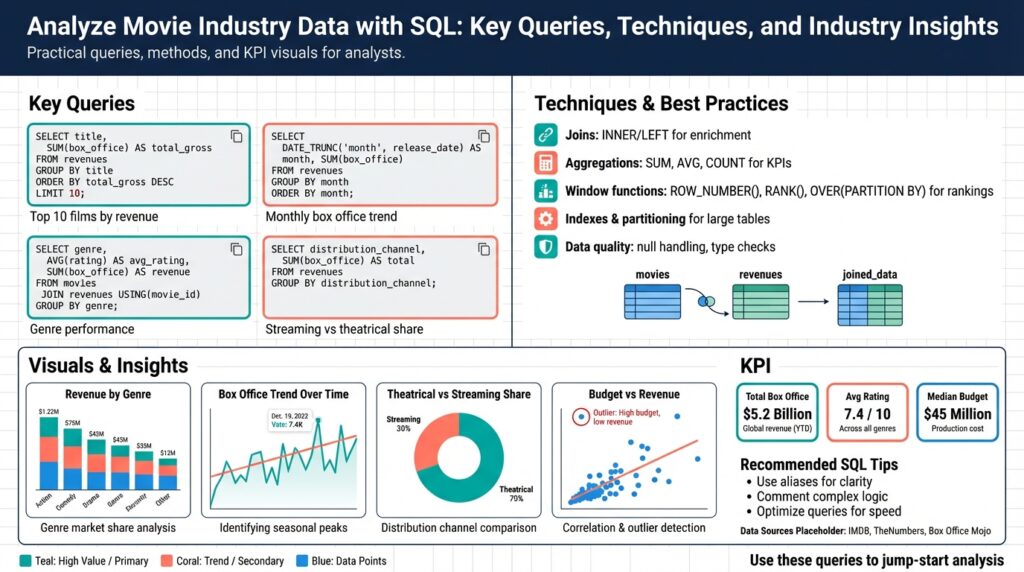
Relationships and keys determine how straightforward your SQL will be. Use integer surrogate keys for joins to minimize index size and reserve original identifiers for lookup columns to preserve provenance. Model cast and crew through credits(movie_id, person_id, role, credited_as) rather than storing arrays — this keeps joins predictable and enables efficient filtering by role. For example, a common analytics pattern is SELECT m.title, SUM(b.gross_usd) AS total_usd FROM movies m JOIN box_office b ON m.movie_id = b.movie_id GROUP BY m.movie_id, m.title; which assumes you normalized currency to a canonical USD amount at ingest.
For analytics you’ll often want a star schema overlay: a dense fact_box_office with measures (gross, screens, admissions) and compact dimension tables like dim_movie, dim_person, dim_date, and dim_territory. This separation accelerates OLAP-style queries and simplifies materialized views. Partition the fact by release_date or reporting_week and cluster or sort by movie_id to reduce I/O when scanning a single title’s run or a week of releases.
Storage and datatype choices matter for both accuracy and performance. Use date and timestamp types for release windows, numeric decimal types for currency to avoid floating-point rounding, and smallint/enums for fixed domain values (release_type, media_type). When you need flexible metadata (alternate titles, distributor-specific fields), store it in a JSONB column and index frequently queried JSON paths. If you expect analytic-scale reads, consider a columnar analytics store (Redshift, BigQuery, ClickHouse) for the fact table while keeping normalized lookup tables in a transactional DB like Postgres.
Data quality and canonicalization are operational concerns you must design for. Normalize person names and create a canonical movie_id to merge duplicates across vendors; maintain lookup tables for territory codes and currency conversion rates; and version ingest pipelines so you can reproduce an aggregated revenue figure. Account for multiple titles, re-releases, and remasters by recording version_id or release_group_id to avoid conflating original runs with later catalogue earnings.
Finally, think about common SQL patterns and performance tricks up front. Precompute running totals in materialized views, maintain weekly pre-aggregations for leaderboard queries, and use partial or expression indexes for typical filters (e.g., WHERE release_date >= current_date - interval '90 days'). How do you keep queries fast when the dataset grows to billions of rows? Combine partition pruning, compact dimension joins, and targeted materialized views to ensure your analytics stay responsive.
With this structure in place, we have a consistent, auditable dataset that supports both ad-hoc exploration and repeatable reports. Next, we’ll translate these modeling decisions into concrete SQL queries and optimization patterns so you can extract business insights from box office, streaming, and audience data quickly and reliably.
Data cleaning and normalization
Building on this foundation, rigorous data cleaning and normalization are the operational plumbing that makes accurate movie analytics possible. You already chose canonical keys and date/currency types; now we enforce those contracts at ingest so downstream SQL behaves predictably. Data cleaning fixes parsing errors, enforces types, and captures provenance; normalization reorganizes denormalized blobs into predictable relations we can join, partition, and aggregate efficiently. Treat these as repeatable ETL steps—idempotent, test-covered, and versioned—so we can reproduce a studio’s reported revenue across pipeline runs.
Start by validating schema and types early in the pipeline so malformed rows never pollute the fact tables. Run tight checks on release_date formats, numeric precision for gross values (use DECIMAL with a fixed scale), and territory codes against a master lookup; reject or quarantine rows that fail instead of silently coercing them. For example, convert string dates to DATE using explicit formats, and store original raw fields as raw_payload or raw_release_date for auditability so you can always trace back why a value changed.
Deduplication and canonicalization for people and titles prevent inflated aggregates and incorrect joins. Create deterministic fingerprints (lowercased, stripped punctuation, normalized whitespace) and use blocking strategies to limit fuzzy-join candidates when matching vendor catalogs. Apply name-canonicalization rules—remove honorifics, normalize diacritics, collapse stage names—and record a canonical_person_id mapping to preserve provenance. When fuzzy matching is ambiguous, surface candidates for human review and store a match_confidence score so analysts can filter joins by reliability.
Normalize multi-valued metadata into associative tables instead of arrays or CSV columns so SQL stays simple and performant. Unnest alternate_titles, distributors, and credits into normalized tables (e.g., movie_titles(title, territory_code, title_type)) and index the foreign keys for joins. If you must keep flexible vendor fields, use a JSONB metadata column and create GIN or expression indexes on commonly queried paths; for example, jsonb_path_exists or jsonb_extract_path_text can be dramatically faster when backed by a targeted index.
Currency and territory normalization deserve special attention: convert local grosses to a canonical currency at ingest and store both the converted value and the original amount/currency. How do you handle historical exchange rates? Maintain a currency_rates(date, currency_code, rate_to_usd) table with effective ranges and apply the rate that corresponds to the release_date or revenue_date. Flag conversions that use estimated or vendor-provided rates and include a conversion_version_id so you can re-run conversions if you later adopt a better FX dataset.
Treat missing values and outliers as first-class citizens rather than hiding them. Use explicit null semantics and add status or quality columns (e.g., gross_usd_is_estimated, release_date_source) so queries can include or exclude data intentionally. For outliers—extremely high grosses or negative values—implement rule-based detectors and store the reason_code when quarantining rows. Preserve original measurements in raw_* columns and maintain a transforms log table that records each change (who/when/why) for auditability and debugging.
Automate validation and normalization so you catch regressions before they reach analytics. Embed unit tests for parsers, CI checks for schema drift, and schema constraints (CHECK, NOT NULL, foreign keys) in the transactional database where feasible. Build a lightweight data-quality dashboard that surfaces failure counts, top failure types, and time-to-fix so ops and analysts can collaborate on persistent issues; when a change in source format breaks revenue ingest, you want a reproducible rollback path rather than ad-hoc fixes.
With clean, normalized data we keep joins simple, aggregations accurate, and provenance intact—enabling reliable leaderboards, cohort analyses, and revenue rollups you can trust. Next, we’ll take these enforced contracts and show concrete SQL patterns and materialized views that exploit the normalized schema for performance and clarity.
Joins and relationship queries
Building on this foundation, the fastest way to unlock insights is to think in relationships rather than tables. We frequently need to answer questions that span movies, people, releases, and time-series metrics, so constructing correct and efficient joins is the everyday work of movie analytics. Start every query by writing the business question in plain language and then map each noun to a canonical table and key—this prevents accidental Cartesian products and keeps join logic auditable and reproducible.
Many practical relationship queries map directly to classic join patterns: inner joins for filtering down to matching entities, left joins for preserving a primary rowset with optional lookups, and semi/anti-joins for existence checks. For example, to list billed actors and their roles you’ll typically join the normalized credits table to movies and persons:
SELECT m.movie_id, m.title, p.person_id, p.name, c.role, c.billing_order
FROM movies m
JOIN credits c ON m.movie_id = c.movie_id
JOIN persons p ON c.person_id = p.person_id
WHERE c.role = 'actor'
ORDER BY m.movie_id, c.billing_order;
This pattern uses surrogate integer keys and small, indexed foreign keys—the exact choices we recommended earlier—to make joins fast and predictable. Use JOIN clauses to express relationships clearly; avoid embedding arrays or JSON lookups for frequent relationship queries because they defeat planner optimizations and make predicate pushdown impossible.
Performance tuning for joins matters when your box_office fact contains millions of rows and credits hold many-to-many mappings. The planner relies on accurate statistics, proper indexes (covering indexes on join keys and common filters), and sensible join ordering; cluster or sort the fact by movie_id to reduce I/O when joining a small dimension. When should you prefer EXISTS or semi-joins over a full join? Use EXISTS for membership checks or to avoid row multiplication when you don’t need dimension columns: it’s often significantly cheaper than distinct-ing after a big join. Always validate assumptions with EXPLAIN ANALYZE and sample queries before promoting patterns to production.
Some relationship queries go beyond flat joins: recursive relationships for franchises and sequel chains, lateral joins for per-title top-N lookups, and window functions for billing and ranking. To get the top three billed cast members per movie you can combine a join with a window function, which is usually faster and clearer than a correlated subquery that aggregates across credits:
SELECT movie_id, title, person_id, name, role
FROM (
  SELECT m.movie_id, m.title, p.person_id, p.name, c.role,
         row_number() OVER (PARTITION BY m.movie_id ORDER BY c.billing_order) rn
  FROM movies m
  JOIN credits c ON m.movie_id = c.movie_id
  JOIN persons p ON c.person_id = p.person_id
) t
WHERE rn <= 3;
Avoid join explosion by isolating multiplicative facts in separate pipelines or by pre-aggregating measures before joining. If you need daily streaming_views summed by movie and platform, aggregate those time-series facts into a compact fact table or materialized view and then join to movie dimensions for reporting. Use lateral joins when you need a small, correlated lookup per row (for example, the highest-grossing release per territory) rather than joining the entire releases table and then grouping.
In practice, instrument your queries: capture runtime metrics, cardinality estimates, and tail latencies so we can spot systematic misestimates in the planner. When relationships are sparse or optional, prefer left joins with explicit null checks and quality flags (e.g., gross_usd_is_estimated) so analysts can filter for reliable data. Finally, balance normalization with pragmatic denormalization—star-schema facts and materialized aggregates accelerate leaderboard and cohort queries, while normalized associative tables keep relationship queries correct and traceable for audit and provenance.
Taking these patterns together, you’ll write relationship queries that are both correct and performant: express relationships with clear joins, choose semi-joins or window functions when appropriate, and pre-aggregate high-cardinality facts to prevent blow-up. Next, we’ll translate these ideas into concrete SQL patterns and optimization recipes that you can apply directly to large box-office and streaming datasets.
Box-office and revenue analysis
Building on this foundation, the first step when interrogating box office revenue is to turn raw time-series facts into business-grade measures you can trust and compare. Start by defining canonical measures—daily_gross_usd, cumulative_gross_usd, and admissions—and store them at the lowest sensible grain (movie_id, release_date, territory_code). When you canonicalize currency at ingest and record conversion_version_id and source_rate_date, you make downstream revenue analytics auditable and reproducible, which is essential for seasonality, cohort, and leaderboard queries.
A practical pattern is to compute running totals with window functions so you can answer questions like “What was this title’s cumulative gross after its fourth weekend?” efficiently and without repeated scans. Implement a materialized view that refreshes nightly and contains cumulative_gross_usd by movie_id and reporting_week; this converts expensive rolling-window work into cheap point-lookup queries. For example, use a query like:
SELECT movie_id, release_date,
       SUM(daily_gross_usd) OVER (PARTITION BY movie_id ORDER BY release_date
                                  ROWS BETWEEN UNBOUNDED PRECEDING AND CURRENT ROW)
       AS cumulative_gross_usd
FROM fact_box_office
WHERE reporting_week >= current_date - INTERVAL '52 weeks';
This pattern gives you both day-level fidelity and precomputed aggregates for leaderboards and cohort rollups.
Reconciling multi-territory reporting and lagged vendor feeds is where many teams lose reliability. How do you reconcile daily grosses across territories with different currencies and reporting cadences? Store both raw_amount and converted_usd alongside a boolean gross_usd_is_estimated and a report_quality_score. Then classify revenue into stable, provisional, and estimated buckets so analysts can filter by confidence. Use a currency_rates table keyed by rate_date to apply the rate that matches the revenue_date; record a conversion_audit row for any retroactive re-rates so historical dashboards can be recomputed deterministically.
When measuring performance, prefer relative metrics and normalized comparisons rather than raw grosses alone. Week-over-week decay rate and per-screen average (PSA) normalize for release scale and provide early signals of long-tail performance. Compute decay as the percentage change in rolling 7-day gross versus the prior rolling 7-day period, and compute PSA as gross_usd / max(screens,1). Those metrics give more actionable insights for distributors deciding on hold/expand strategies than a top-line gross number.
Detecting anomalies and attribution errors requires integrated quality signals and lightweight audit joins. Build a transforms_log table that records each ETL change (who, when, why) and join it to suspicious rows for rapid triage. For attribution—allocating gross back to distributors, exhibitors, and revenue types—use release_group_id and revenue_share rules applied in a dedicated allocation step rather than ad-hoc SQL during reporting. Precompute allocated_revenue into a compact fact table to speed downstream P&L queries and to prevent repeated floating-point adjustments in dashboards.
Finally, instrument and iterate: capture query latency, cardinality estimates, and tail errors for your top 20 dashboard queries and maintain weekly pre-aggregations for trending windows (7d, 28d, 52w). Taking these steps turns large-scale movie data into reliable insights you can operationalize—real-time leaderboards, territory-level forecasts, and finance-grade revenue rollups—while keeping the system auditable and performant. Building on these patterns, next we’ll translate them into concrete SQL templates and materialized views you can drop into an analytics schema.
Ratings and audience insights
Ratings are one of the quickest levers for extracting audience insights, but they’re also one of the trickiest signals to interpret at scale. We often see teams treat average_score as gospel; instead, start by asking a simple question: how do you know whether a high average rating reflects broad approval or a small, enthusiastic sample? Building on the normalized schema we described earlier, treat ratings as a first-class time-series fact (rating_value, movie_id, user_id, rating_date, rating_source, rating_confidence) so you can join, partition, and aggregate them reliably for downstream analysis.
Modeling and querying rating metrics should be straightforward and auditable. Store raw user ratings alongside a canonical converted score where necessary (e.g., normalize 5-star, 10-point, and thumbs systems to a 0–100 scale) and preserve the original payload for provenance. A practical starting query computes the aggregate and distribution per title and platform; for example:
SELECT m.movie_id, m.title,
       COUNT(r.rating_value) AS n_ratings,
       AVG(r.normalized_score) AS avg_score,
       SUM(CASE WHEN r.normalized_score >= 80 THEN 1 ELSE 0 END) AS top_box
FROM movies m
JOIN ratings r ON m.movie_id = r.movie_id
WHERE r.rating_date >= current_date - INTERVAL '365 days'
GROUP BY m.movie_id, m.title;
Raw aggregates are useful, but you must correct for sampling variance and bias. Ratings are sensitive to selection effects (early adopters, review-bombing) and small-n volatility, so apply Bayesian shrinkage or Empirical Bayes to stabilize estimates for low-count titles. Define a prior (global mean mu and a strength alpha) and compute a posterior mean; in SQL this looks like:
SELECT movie_id,
       (SUM(normalized_score) + :alpha * :mu) / (COUNT(*) + :alpha) AS shrunk_score,
       COUNT(*) AS n_ratings
FROM ratings
GROUP BY movie_id;
This technique reduces false positives in leaderboards and gives you a principled way to rank films early in a release window.
Beyond central tendency, inspect the full rating distribution and its evolution over time to uncover shifts in sentiment. Use window functions to compute rolling medians, percentiles, and week-over-week drift; materialize these as nightly aggregates so analysts and dashboards don’t repeatedly scan billions of rows. For example, a 7-day rolling average and the percentage change from the prior week reveal whether a title is gaining or losing audience momentum—information that directly impacts marketing spend and release scheduling.
To generate richer audience insights, join ratings to audience demographics and engagement signals (streaming_views, dwell_time, rewatch_rate). Segment by cohort (age_bucket, region, subscription_tier) and compute conditional metrics: average_score by cohort, conversion rate from trial-to-paid among high scorers, or retention among viewers who rated above a threshold. These cross-tabs tell you not just whether people liked a movie, but who liked it and how that liking correlates with monetizable behavior—exactly the input product and distribution teams need when deciding on promotion, territory expansion, or catalogue positioning.
Operationalize quality and provenance so business users can trust the signals. Tag ratings with source weights (platform credibility), quality flags (bot_detected, duplicate_user), and a confidence score derived from user history; then surface only high-confidence metrics in finance-grade reports. For performance, partition the ratings fact by rating_date and cluster by movie_id, and maintain nightly materialized views for leaderboards, percentile bands, and per-cohort aggregates to keep interactive queries fast.
Taking these steps turns noisy user feedback into actionable audience insights and reliable KPIs for programming, marketing, and personalization. In the next section we’ll translate these stabilized rating metrics into concrete SQL templates and dashboard patterns you can drop into a reporting schema for automated leaderboards and forecast inputs.
Time-series and trend detection
Building on this foundation, think of time-series and trend detection as the backbone of operational movie analytics: you need SQL patterns that expose momentum, not just point-in-time totals. Time-series and trend detection should appear early in your reporting pipeline so you can answer business questions like “Is this title’s box-office still accelerating or already in long-tail decay?” quickly and reproducibly. Front-load daily and weekly grains in the fact tables (fact_box_office, streaming_views) and use date dimensions for consistent bucketing; this lets SQL optimizers prune partitions and keeps rolling calculations efficient.
Start with basic, robust primitives that reveal short- and medium-term trends. Use window functions to compute rolling averages, week-over-week change, and LAG-based deltas so you can triage titles by momentum. For example, a 7-day rolling average of daily gross highlights emerging winners while smoothing noise:
SELECT movie_id, release_date,
  AVG(daily_gross_usd) OVER (PARTITION BY movie_id ORDER BY release_date ROWS BETWEEN 6 PRECEDING AND CURRENT ROW) AS ma7
FROM fact_box_office
WHERE release_date BETWEEN :start AND :end;
This pattern surfaces trend detection signals quickly and scales when you prefilter to active releases. For campaign decisions we also compute week-over-week decay as a relative change between two rolling windows so you compare momentum across titles with different launch shapes.
Move beyond simple smoothing when you need directional confidence. Use LAG/LEAD to detect persistent slope and combine with count thresholds to avoid small-n noise. For example, flag a positive trend only when the 7-day rolling average has increased for three consecutive measurement points and daily sample size exceeds a minimum: this reduces false positives from reporting lags or patchy vendor feeds. When your SQL engine supports regression aggregates (Postgres’s regr_slope or equivalent), compute a local linear trend inside a window to quantify the slope and its significance rather than relying on brittle percentage changes.
Detecting anomalies and attribution issues requires mixing quality signals with the raw metric. Join gross rows to report_quality flags (gross_usd_is_estimated, source_lag_days) and exclude provisional data from trend detection or downgrade its confidence. Implement a simple cumulative-sum change-point test in SQL by computing residuals versus a recent baseline and then scoring sequences of positive residuals; flag sequences that exceed a threshold for human review. For complex statistical methods—seasonal decomposition or STL smoothing—export sampled time-series from SQL to a Python or R job and feed the results back as diagnostics or adjusted series in a compact analytics table.
Operational patterns matter as much as algorithms. Materialize nightly aggregates (daily, weekly, 28-day) into a compact trend_facts table and refresh it with incremental inserts to keep dashboards responsive. Partition trend_facts by reporting_week and cluster by movie_id so per-title lookups are cheap. Maintain a transforms_log that records which conversion_rate and aggregation_version produced each trend metric so you can recompute or backfill deterministically when FX or attribution rules change.
How do you act on these signals? Integrate trend detection into automated rules for distribution: expand screens or push marketing when the slope and volume both pass thresholds; conversely, pause paid acquisition for titles with sustained negative decay. Present trend confidence alongside raw numbers in dashboards so product and finance teams can weigh provisional data appropriately. Taking these steps converts time-series into actionable insight—fast, auditable, and tuned to the realities of box office and streaming data—and prepares you to implement production-grade SQL templates and materialized views in the next section.
