Overview of Aggregate Functions
Aggregate functions are the workhorses you reach for when you need a single summary value from many rows, and they shape how you design reporting queries and OLAP pipelines. Building on what we covered earlier about relational schemas and normalization, we now treat aggregation as a distinct layer: compute summaries with SUM, COUNT, and AVG, then join or store those results for downstream use. These aggregate functions condense row-level detail into metrics you can act on, and choosing the right one affects correctness, performance, and maintainability from day one.
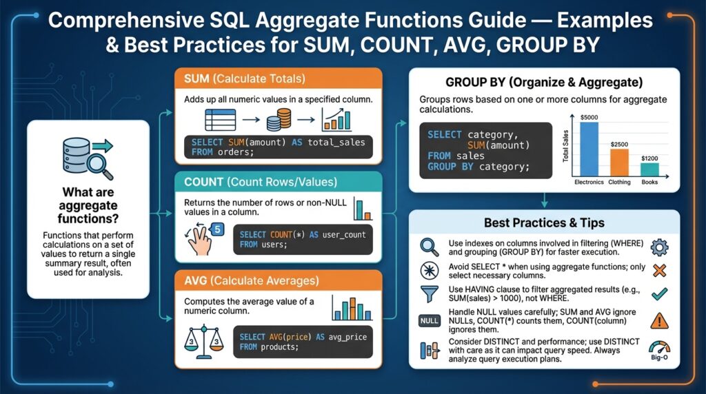
At a conceptual level, each aggregate function reduces a set of input values to one output value over a grouping scope. For example, SUM totals numeric values, COUNT counts rows or non-null values, and AVG computes an arithmetic mean. You express the scope with GROUP BY — for instance, grouping by customer, date, or geographic region — and the query planner applies the aggregate across each group. Practically, you write queries like:
SELECT customer_id, SUM(amount) AS total_spend
FROM payments
WHERE status = 'settled'
GROUP BY customer_id;
This pattern is the starting point for dashboards, billing jobs, and SLA reports because it converts streaming event rows into human-readable KPIs.
How do you decide when to use COUNT() versus COUNT(column) or COUNT(DISTINCT column)? The choice determines what you count. COUNT() counts rows (including rows with nulls), COUNT(column) counts only non-null column values, and COUNT(DISTINCT column) deduplicates before counting. In a payments table, COUNT(*) gives the number of transactions, COUNT(payment_method) excludes records missing that field, and COUNT(DISTINCT card_hash) estimates unique cards used. Use COUNT(DISTINCT) sparingly on high-cardinality fields because it can be expensive; many OLAP systems offer approximate distinct algorithms when you need speed over absolute precision.
Numeric aggregates have semantic and implementation quirks you must handle deliberately. SUM and AVG on integer columns can overflow or produce integer division truncation depending on the engine, so cast to a wider or decimal type when necessary:
SELECT AVG(amount::numeric) AS avg_amount
FROM payments;
Moreover, AVG is computed as SUM/COUNT in many implementations, so be mindful of nulls and filtering: applying WHERE before aggregation differs from filtering inside a conditional aggregate (e.g., SUM(CASE WHEN status = ‘settled’ THEN amount ELSE 0 END)). These patterns let you compute multiple metrics in one scan with predictable semantics.
GROUP BY enforces discipline around which columns appear in the result set: any non-aggregated column must be part of the group key. This is both a correctness guard and a performance lever — the group key determines sort/hash work and parallelization. When you need row-level detail alongside aggregates, use window functions instead of flattening groups and joining back, because window functions compute aggregates over partitions without collapsing rows, preserving detail and avoiding extra joins.
Performance considerations are practical constraints, not optional optimization hobbies. Indexes that cover the group key and the aggregated column can drastically reduce I/O; materialized views, pre-aggregated tables, or incremental aggregation jobs reduce query latency for large datasets. For streaming workloads, adopt incremental or rollup strategies (hourly/daily aggregates) to avoid re-scanning raw events for every report. When COUNT DISTINCT or heavy GROUP BY workloads become bottlenecks, consider approximate algorithms or distributed aggregation frameworks.
Common pitfalls include unexpected null-handling, implicit type coercion, and group cardinality explosions when you group by high-cardinality columns like timestamps or unique identifiers. Test aggregations with representative datasets and edge cases — nulls, sparse data, and skewed distributions — because correctness in production often fails for the same reasons as performance does: data shape. Taking this approach ensures your aggregations remain reliable, performant, and maintainable as the system scales, and sets us up to dig into practical examples and best practices for SUM, COUNT, AVG, and GROUP BY in the next section.
SUM, COUNT, AVG Examples
Building on this foundation, practical examples show how SUM, COUNT, and AVG drive real reporting queries and OLAP pipelines. In the next examples we’ll assume a payments table with columns (id, customer_id, amount, status, created_at, card_hash) and show patterns you will use daily: conditional aggregation, filtered aggregates, precision-safe calculations, and windowed averages. These patterns reduce multiple scans, avoid null-related surprises, and keep group keys small so queries remain performant.
Use conditional aggregation to compute multiple related metrics in one scan. For example, to get total settled spend, refunded spend, and number of settled transactions per customer in a single query you can write either the CASE form (ANSI-compatible) or the FILTER form (PostgreSQL-style):
SELECT
  customer_id,
  SUM(CASE WHEN status = 'settled' THEN amount ELSE 0 END) AS total_settled,
  SUM(CASE WHEN status = 'refunded' THEN amount ELSE 0 END) AS total_refunded,
  COUNT(*) FILTER (WHERE status = 'settled') AS settled_count
FROM payments
GROUP BY customer_id;
This approach reduces I/O because the planner scans the table once and computes SUM and COUNT over the same group key. Note that we used a zero fallback inside SUM to preserve numeric semantics; if you instead need nulls to indicate absence, use NULL in the ELSE branch and be explicit about handling later. Also remember to cast amount to a wider type to avoid overflow or integer truncation: SUM(amount::numeric) or SUM(amount::bigint) depending on your data.
When you need accurate distinct counts, weigh cost vs. precision. COUNT(DISTINCT card_hash) gives the exact number of unique cards per customer but can be expensive on high-cardinality fields. If you must scale, many data warehouses offer approximate distinct functions (for example, APPROX_COUNT_DISTINCT or HyperLogLog-based aggregates) that trade small error for much less memory and CPU. How do you decide? Use exact COUNT(DISTINCT) for billing or compliance; use approximate distinct for analytics dashboards where performance matters more than a few percentage points of error.
AVG is often implemented as SUM/COUNT, so you can compute aggregate averages alongside conditional metrics without extra passes. To compute a weighted average—say, average amount per day weighted by transaction count—we compute sums and counts explicitly and divide with proper casting to preserve decimal precision:
SELECT
  date_trunc('day', created_at) AS day,
  SUM(amount)::numeric / NULLIF(COUNT(*), 0) AS avg_amount,
  SUM(amount) FILTER (WHERE status = 'settled')::numeric / NULLIF(COUNT(*) FILTER (WHERE status = 'settled'), 0) AS avg_settled
FROM payments
GROUP BY day;
When you need row-level detail plus aggregates, prefer window functions over joining group results back to the base table. For example, to annotate each transaction with the customer’s running AVG amount over the last 30 days, use:
SELECT *, AVG(amount) OVER (PARTITION BY customer_id ORDER BY created_at RANGE BETWEEN INTERVAL '30 days' PRECEDING AND CURRENT ROW) AS avg_30d
FROM payments;
Finally, focus on practical performance: create indexes that cover the group key and the filtered predicate (e.g., partial indexes for status = ‘settled’), pre-aggregate into daily/hourly materialized tables for heavy dashboards, and test with realistic skewed distributions. These examples show how SUM, COUNT, and AVG combine into compact, efficient metrics that you can materialize, query with window functions, or expose to downstream jobs. Taking these patterns into your pipelines will make aggregations both correct and performant as data volume grows.
GROUP BY Usage and Examples
Building on this foundation, GROUP BY is where you convert row-level events into the concrete metrics you ship to dashboards and billing jobs, and choosing the right grouping strategy directly affects correctness and performance. GROUP BY determines the aggregation scope — which rows collapse into each summary — so front-load your group keys with the most meaningful dimensions (customer, day, region) and avoid grouping on high-cardinality identifiers unless you actually need per-entity metrics. How do you decide the right granularity for a report? Think about query patterns, retention needs, and whether downstream consumers expect rollups or raw per-entity counts.
Use grouping expressions when the natural key in your schema doesn’t match the reporting granularity. Date bucketing is the most common example: grouping by date_trunc(‘day’, created_at) or by a generated date column reduces group cardinality and improves planner choices, and we should prefer persisted date keys for very large tables. When you need multiple rollup levels — daily and monthly, or customer and product — consider ROLLUP, CUBE or GROUPING SETS to compute several groupings in a single scan rather than issuing multiple queries; these features reduce I/O and keep aggregates consistent across levels.
When should you use ROLLUP or GROUPING SETS instead of multiple queries? Use them whenever you need hierarchical or combinatorial summaries from the same dataset. For example, ROLLUP(customer_id, date_trunc(‘month’, created_at)) produces per-customer-per-month, per-customer, per-month, and grand totals in one pass. The SQL looks like:
SELECT
  customer_id,
  date_trunc('month', created_at) AS month,
  SUM(amount) AS total_amount
FROM payments
GROUP BY ROLLUP(customer_id, month);
This pattern keeps totals consistent and avoids the join complexity of separately computed aggregates. Be explicit about NULL interpretation: ROLLUP uses NULL to signal a rolled-up level, so annotate results or use GROUPING() functions where supported to distinguish real NULL keys from rollup placeholders.
Filter groups with HAVING, not WHERE, because WHERE limits input rows while HAVING applies after aggregation. Use HAVING to enforce metrics-level conditions, for example to exclude customers whose settled_count is below a threshold: HAVING COUNT(*) FILTER (WHERE status = ‘settled’) > 10. Also prefer computed predicates in HAVING to avoid an extra aggregation pass: the planner can combine them efficiently when you express the computation inside the aggregate or reuse filtered aggregates.
Grouping across joins requires intent: decide whether to aggregate pre- or post-join. When the join multiplies rows (for example, joining orders to many line_items), pre-aggregate the multiplicative side to its natural grain and then join the smaller summary to avoid explosion. For instance, aggregate line_items by order_id first, compute SUM(qty) and SUM(qty*price), then join to orders to GROUP BY customer_id. This reduces memory pressure and avoids incorrect double-counting.
Performance tuning for GROUP BY is pragmatic: create indexes on the group key and any filtered predicate (including partial indexes for status=’settled’), consider clustering or partitioning by time when aggregating over date ranges, and materialize heavy rollups as daily/hourly tables for dashboards. When you face skewed group distributions, use sampling or approximate distinct functions for analytics (but keep exact counts for billing/compliance). Also profile whether your engine prefers hash aggregation or sort-based aggregation and adjust work_mem, parallelism, or grouping strategies accordingly.
Finally, make your GROUP BY queries maintainable by naming expressions, using conditional aggregates, and annotating rollup rows so consumers can parse hierarchy reliably. Taking this approach ensures your aggregation logic scales with data volume while remaining auditable and fast, and prepares you to apply window functions or incremental materialization patterns in the next section.
HAVING vs WHERE Filters
Building on this foundation, many developers stumble over the difference between WHERE and HAVING when they first write GROUP BY queries. HAVING and WHERE are both filters, but they operate at different stages of query processing: WHERE filters input rows before any aggregation, while HAVING filters the resulting groups after aggregates are computed. Getting this wrong produces silent correctness bugs—incorrect counts, unexpected NULLs, or costly full-table scans—so we’ll make the distinction concrete and practical. How do you decide which to use and how to combine them for both correctness and performance?
At the simplest level, WHERE is a row-level predicate and HAVING is a group-level predicate. WHERE cannot reference aggregate functions because it runs before aggregation; HAVING can reference aggregates because it runs after GROUP BY produces a single row per group. For example, to find customers with more than ten settled transactions you might write either of these patterns:
-- filter rows first, then group
SELECT customer_id, COUNT(*) AS settled_count
FROM payments
WHERE status = 'settled'
GROUP BY customer_id
HAVING COUNT(*) > 10;

-- group then filter using an aggregate that encodes the predicate
SELECT customer_id, COUNT(*) AS settled_count
FROM payments
GROUP BY customer_id
HAVING COUNT(*) FILTER (WHERE status = 'settled') > 10;
Both are valid, but they express different intents and have different performance characteristics. The first query uses WHERE to prune rows early (reducing I/O and the work the aggregator must do) and then applies HAVING to the aggregated result; the second computes the aggregate across all rows in the group and then filters groups by the filtered-COUNT expression. In practice prefer WHERE when the predicate is purely row-level (for example, status, created_at ranges, or join conditions) because it enables index usage and partition pruning in most engines.
There are practical edge cases and portability issues to watch for. Some databases (notably older MySQL configurations) permit non-aggregated columns in HAVING without listing them in GROUP BY, which is a non-ANSI extension and causes non-deterministic results; rely on ANSI semantics for predictable behavior across engines. Also remember that HAVING without GROUP BY aggregates the whole table into one row and then filters it, which can be useful when you want a global check (for example, HAVING SUM(amount) > 1000000) but will be confusing if you expect per-entity filtering. Optimizers sometimes rewrite queries to push predicate logic earlier, but you should not rely on rewrites for correctness—only for potential performance improvements.
When you need multiple related metrics in one scan, conditional aggregates are a powerful pattern that reduces the need for multiple HAVING clauses or separate scans. For instance, compute per-customer totals and settled counts in one pass and then apply a HAVING that references those computed aggregates:
SELECT customer_id,
       SUM(amount) FILTER (WHERE status = 'settled') AS total_settled,
       COUNT(*) FILTER (WHERE status = 'settled') AS settled_count
FROM payments
WHERE created_at >= '2025-01-01' -- row-level prune
GROUP BY customer_id
HAVING COUNT(*) FILTER (WHERE status = 'settled') > 10;
This pattern keeps scanning cost low (WHERE) while expressing metric-level constraints in HAVING. In real-world pipelines you’ll often combine WHERE for data-quality and join predicates and HAVING for business-rule thresholds (for example, exclude customers with low transaction volume from downstream billing). Be mindful of NULL handling and numeric types when you aggregate—cast as needed before applying HAVING.
To summarize the checklist you can apply immediately: use WHERE to reduce input rows and enable indexes or partition elimination; use HAVING to enforce post-aggregation rules that reference computed metrics; prefer conditional aggregates when computing multiple metrics in one scan; and avoid relying on non-ANSI HAVING behaviors for portability. Taking these patterns into your queries will keep aggregates correct, performant, and maintainable as data shapes and scale evolve, and prepares us to compare these approaches with window functions and materialized rollups next.
Handling NULLs in Aggregations
Building on this foundation, null handling is one of the most frequent sources of subtle bugs in production aggregations, and you should front-load the semantics: most SQL aggregate functions ignore NULL inputs, while COUNT(*) counts rows regardless of NULLs. When you write aggregation queries, make null handling an explicit design decision because downstream dashboards, billing jobs, and alerts will interpret a missing value differently than an explicit zero. How do you decide whether an absent value should be treated as zero, unknown, or excluded from a metric? The answer depends on business intent and the contract you expose to consumers.
At the SQL level the rules are straightforward but important to remember. SUM, AVG, and MAX/MIN skip NULL inputs; SUM over only NULLs returns NULL, not 0, and COUNT(column) counts only non-null entries while COUNT(*) counts rows. You can make that behavior explicit with simple constructs: for example, choose between a filtered aggregate that yields NULL when nothing matches and a CASE/ELSE that yields 0:
-- NULL when no settled rows exist
SELECT customer_id, SUM(amount) FILTER (WHERE status='settled') AS settled_sum
FROM payments GROUP BY customer_id;

-- 0 when no settled rows exist
SELECT customer_id, SUM(CASE WHEN status='settled' THEN amount ELSE 0 END) AS settled_sum
FROM payments GROUP BY customer_id;
Use COALESCE to normalize result-level nulls when you need a stable numeric contract (for example, COALESCE(SUM(…), 0)). That pattern is useful for dashboards or export pipelines that expect numeric fields rather than nullable types.
AVG deserves special attention because many engines implement it as SUM/COUNT. If you compute an average by hand, guard against division-by-zero and null propagation: cast to a decimal for precision and use NULLIF to avoid dividing by zero, then COALESCE if you need a default. For example:
SELECT
  customer_id,
  COALESCE(SUM(amount)::numeric / NULLIF(COUNT(amount), 0), NULL) AS avg_amount
FROM payments
GROUP BY customer_id;
This preserves the semantic distinction between “no data” (NULL average) and “zero average” (0.0) depending on your business rule. If you want 0.0 when there are no values, wrap the division in COALESCE(…, 0).
Choosing when to preserve NULLs versus collapsing them to zeros is a policy decision with real consequences. For SLA or billing metrics you often prefer 0 to indicate no activity; for data-quality checks or anomaly detection you may prefer NULL to flag missing data that warrants investigation. Treat the choice as part of your metric contract: document it, implement it consistently (either at query-time with COALESCE/CASE or upstream during ingestion), and include unit tests that assert behavior on edge-case datasets.
Nullable grouping keys and rollups introduce another class of traps. Grouping by a nullable column produces a NULL bucket for missing keys, and ROLLUP uses NULL to represent higher-level aggregates. To make buckets explicit, normalize keys with COALESCE in the GROUP BY or use GROUPING() (where supported) to distinguish real NULLs from rollup placeholders. For example, GROUP BY COALESCE(region, ‘UNKNOWN’) avoids an implicit NULL group and makes downstream joins and visualizations simpler.
From an operational standpoint, be deliberate and test-driven: simulate groups with no matching rows, sparse distributions, and extreme skews; assert your aggregation outputs (NULL vs 0) in automated tests; and document the chosen null semantics in metric schemas. Taking this concept further, we’ll apply these null-handling patterns to windowed aggregates and incremental materializations so metrics remain both correct and predictable as volume grows.
Window Functions vs Aggregates
Building on this foundation, choosing whether to collapse rows into group-level summaries or preserve per-row context is one of the most consequential design decisions you make when shaping metrics. If you need a single metric per entity—total spend per customer or daily unique counts—aggregate functions and GROUP BY are the natural fit because they reduce data early and make results compact. If you need to annotate each event with contextual metrics—running totals, percent-of-group, or lagged comparisons—window functions let you compute those without collapsing rows. When should you collapse and when should you preserve row-level context? That question drives both correctness and performance trade-offs.
At a conceptual level the difference is straightforward: aggregates fold many rows into one row per group, while window functions compute values over a partition yet leave the original rows intact. Aggregates (SUM, COUNT, AVG) paired with GROUP BY produce a result set with one row per group key and are ideal when the consumer expects rolled-up metrics. Window functions use PARTITION BY and an optional ORDER BY and frame clause to produce a value for every input row—this is how you attach moving averages, ranks, or percentiles to raw events without a separate join step.
Concrete SQL illustrates the distinction. To get daily spend per customer you write a GROUP BY query that reduces rows:
SELECT customer_id, date_trunc('day', created_at) AS day, SUM(amount) AS total_day
FROM payments
GROUP BY customer_id, day;
To annotate every transaction with that customer’s 30-day running average without collapsing rows you use a windowed aggregate:
SELECT *,
  AVG(amount) OVER (PARTITION BY customer_id ORDER BY created_at
                    RANGE BETWEEN INTERVAL '30 days' PRECEDING AND CURRENT ROW) AS avg_30d
FROM payments;
Both return useful metrics, but they answer different questions and support different downstream workflows.
Performance characteristics differ and should influence your decision. Aggregates allow hash or sort-based grouping that can be parallelized and pushed down through filters (WHERE) and index scans, so they often win when you’re summarizing large tables into a compact result. Window functions commonly require sorting each partition and maintaining frame state; that work can be expensive when partitions are large or ORDER BY uses high-cardinality keys. To optimize windowed queries, limit partition sizes (partition by date or shard keys), add appropriate indexes to support the ORDER BY, and avoid overly wide frames when a bounded window suffices.
In real systems we frequently combine both approaches to balance correctness and cost. Pre-aggregate high-volume event streams into daily/hourly rollups with aggregates and use window functions on those smaller tables to compute trends or rolling windows—this reduces I/O and memory pressure. For example, materialize daily customer totals with aggregates and then run windowed percent change over the last 7 daily rows to produce a stable time-series indicator. This pattern gives you the compactness of aggregates and the per-row insights window functions provide, while keeping queries predictable and performant.
There are important semantic gotchas to watch for when mixing patterns. GROUP BY enforces which columns appear in the result and hides row-level variance, so don’t expect to recover individual event attributes after aggregation without a join. Window functions preserve row count but require deterministic ordering if you rely on frames that use PRECEDING/UNBOUNDED—omitting a clear ORDER BY can lead to non-deterministic results. Also note that COUNT(DISTINCT) is straightforward in aggregate queries but rarely available as a windowed distinct; you’ll often need workarounds (subqueries, approximate functions) when you need per-row distinct-cardinality context.
To decide quickly in practice, follow a simple heuristic: use aggregates and GROUP BY when the metric’s contract is one row per entity or time bucket and you can prune early with WHERE; use window functions when you must enrich each row with context like running sums, ranks, or lag/lead comparisons. When both are needed, pre-aggregate and then apply window functions to the reduced dataset. Taking this approach lets us design queries that are correct, maintainable, and efficient, and prepares us to apply incremental materialization and partitioning strategies in the next section.