Quick overview: What is a CNN
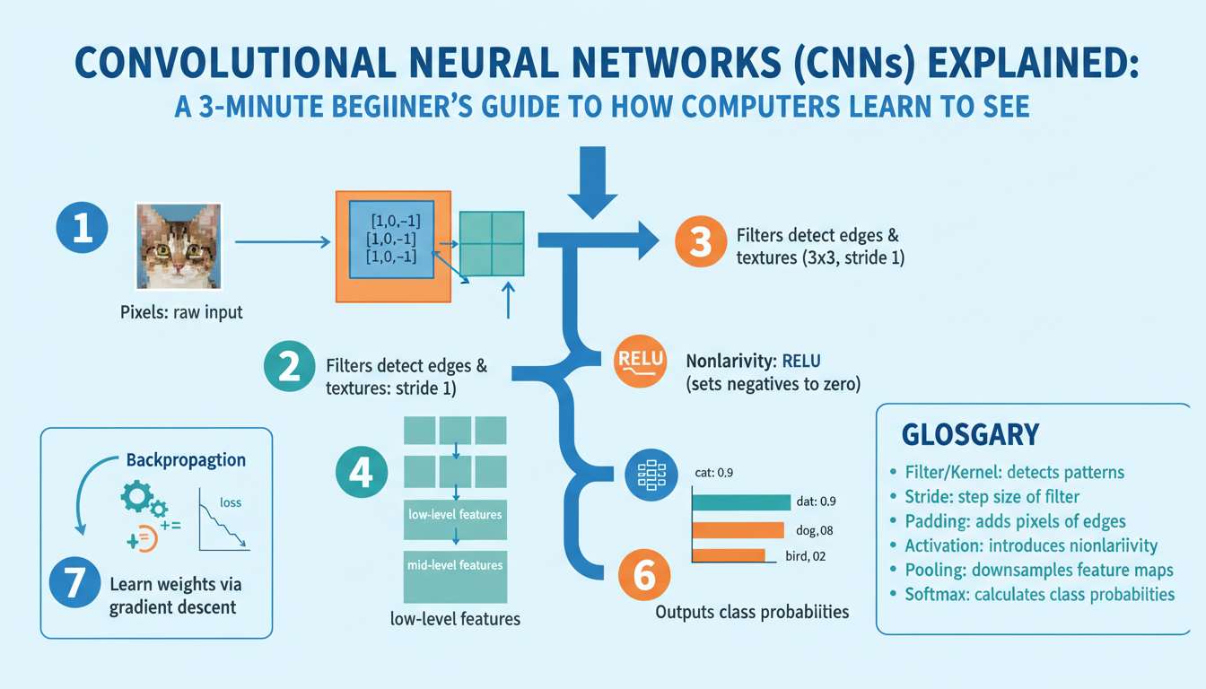
Convolutional neural networks are a type of deep learning model built to process grid-like data (most commonly images). Instead of treating every pixel independently, they apply small learnable filters that slide across the image to detect local patterns—edges, textures, and simple shapes—producing feature maps that highlight where those patterns occur.
Key ideas are local connectivity and weight sharing: each filter looks at a small neighborhood, and the same filter is reused across the whole image, which drastically reduces parameters and helps the model generalize. Nonlinear activations (e.g., ReLU) follow convolutions to capture complex relationships. Pooling or strided convolutions reduce spatial resolution, giving some translation invariance and lowering computation.
As depth increases, layers compose simple features into higher-level concepts (edges → motifs → object parts). A final pooling/fully connected head converts learned features into predictions. CNNs are trained end-to-end with backpropagation and gradient-based optimization on labeled data, and they power tasks like image classification, object detection, and segmentation due to their efficiency and ability to learn hierarchical visual representations.
Intuition: How CNNs see images
Imagine an image as a stack of tiny neighborhoods. Small learnable filters (kernels) slide over those neighborhoods and respond strongly when a specific local pattern appears — a vertical edge, a color contrast, or a tiny curve. Each filter produces a feature map that says “where” that pattern occurs. Because the same filter is reused across the whole picture (weight sharing), the network recognizes the same pattern anywhere in the image, giving translation robustness while keeping the model compact.
Early layers act like simple visual detectors: edges, color blobs, gradients. Intermediate layers combine those detectors into motifs and textures: corners, repeating stripes, or parts of objects. Deeper layers compose motifs into semantic concepts: eyes, wheels, or entire faces. Nonlinear activations (e.g., ReLU) between convolutions let the network mix and amplify useful patterns, while pooling or strided convolutions reduce spatial size so later layers focus on larger contexts.
The key intuition is hierarchical composition: complex visual ideas are built by repeatedly combining simpler ones, with each neuron having a growing receptive field that sees more of the image. Visual tools like activation maps and filter visualizations let you peek into which patterns a network has learned, revealing why a prediction was made rather than leaving the model as a black box.
Convolution operation — step by step
Think of convolution as a small filter scanning an image and computing a single number at each position: place the kernel over a patch, multiply corresponding elements, sum them, add a bias, then (optionally) apply an activation. Move the kernel by the stride and repeat; padding controls whether edges are included.
Example (stride=1, no padding). Input image:
[ [1, 2, 0],
  [0, 1, 3],
  [2, 1, 0] ]
Kernel:
[ [1, 0],
  [0, -1] ]
Compute at top-left patch: 11 + 20 + 00 + 1(-1) = 0. Top-right: 21 + 00 + 10 + 3(-1) = -1. Bottom-left: 01 + 10 + 20 + 1(-1) = -1. Bottom-right: 11 + 30 + 10 + 0(-1) = 1. Feature map before activation: [[0, -1], [-1, 1]]. After adding bias (if any) and applying ReLU, negatives become 0, giving [[0, 0], [0, 1]].
For multi-channel inputs, each filter has the same depth as the input; multiply and sum across channels, then sum those results to produce one spatial value. Stacking many different filters produces multiple feature maps that capture different patterns. Stride >1 downsamples; “same” padding preserves spatial size; “valid” means no padding. This elementwise multiply-and-sum plus weight sharing is the core operation that lets CNNs detect local patterns efficiently.
Filters, kernels, and feature maps
Filters are small, learnable weight arrays (kernels) that scan an image patch-by-patch and compute a dot product to measure how well a local pattern matches. Because the same filter is reused across spatial locations (weight sharing), a single kernel can detect the same feature—an edge, a texture, or a color blob—anywhere in the image while keeping parameter count low. After each dot-product, an optional bias and nonlinearity (e.g., ReLU) turn raw responses into useful signals.
For multi-channel inputs (RGB or earlier feature stacks), each filter has the same depth as the input: it multiplies and sums across channels at every spatial location, producing one scalar per position. Stacking many distinct filters in a layer yields a set of feature maps—one map per filter—that highlight where each learned pattern appears. Stride and padding control spatial sampling and output size.
Early feature maps are interpretable (edges, color blobs); deeper maps become abstract, combining lower-level maps into motifs and object parts. Inspecting these maps helps diagnose what the network has learned and guides architectural choices like filter size and layer depth.
Pooling and downsampling explained
Reducing spatial size is a core tool in CNNs: it lowers computation, grows each neuron’s receptive field, and adds a bit of translation robustness by discarding tiny shifts. The two simplest, widely used operations are max pooling and average pooling. Max pooling picks the strongest activation inside a local window (often 2×2) and preserves the most salient feature; average pooling computes the mean and yields a smoother, lower-resolution summary. A common 2×2 max-pool with stride 2 turns this 4×4 patch into a 2×2 map by taking the maximum in each non-overlapping window.
Example (2×2 windows):
Input patch:         After 2×2 max-pool:
[ [1, 3, 2, 0],        [3, 2]
  [0, 2, 1, 4],  ->    [2, 4] ]
Global pooling reduces each feature map to a single value (useful before classifiers), while overlapping pooling uses smaller strides to retain more spatial info.
Downsampling can instead be achieved by strided convolutions, which are learnable and often preserve richer information than fixed pooling. The trade-off is complexity and extra parameters. Pooling is simple, parameter-free, and effective for aggressive size reduction; strided convs give the network control over what to keep.
Be mindful: pooling increases invariance but discards precise location—bad for tasks needing fine spatial detail (e.g., segmentation). Modern designs mix short strided convs, occasional pooling, or replace pooling with learned downsampling depending on the task and computational budget.
Build a tiny CNN example
Below is a minimal PyTorch example that shows the core pieces: small convolutional stack, pooling, a classifier head, and a single training step. Input size assumed 32×32 RGB, 10 classes.
import torch
import torch.nn as nn
import torch.nn.functional as F

class TinyCNN(nn.Module):
    def __init__(self, num_classes=10):
        super().__init__()
        self.conv1 = nn.Conv2d(3, 8, kernel_size=3, padding=1)   # 32x32 -> 32x32
        self.conv2 = nn.Conv2d(8, 16, kernel_size=3, padding=1)  # 16 feature maps
        self.pool = nn.MaxPool2d(2, 2)                           # halves spatial dims
        self.fc = nn.Linear(16 * 8 * 8, num_classes)             # after two pools

    def forward(self, x):
        x = F.relu(self.conv1(x))
        x = self.pool(x)           # 32 -> 16
        x = F.relu(self.conv2(x))
        x = self.pool(x)           # 16 -> 8
        x = torch.flatten(x, 1)
        return self.fc(x)

# quick run
model = TinyCNN(num_classes=10)
optimizer = torch.optim.SGD(model.parameters(), lr=0.01)
criterion = nn.CrossEntropyLoss()

# dummy batch: batch_size=4, 3x32x32
images = torch.randn(4, 3, 32, 32)
labels = torch.randint(0, 10, (4,))

# forward + single training step
logits = model(images)
loss = criterion(logits, labels)
optimizer.zero_grad()
loss.backward()
optimizer.step()

print(f"Loss: {loss.item():.4f}")
This tiny model demonstrates the convolution→ReLU→pool pattern, progressive channel growth, and how spatial dimensions shrink. For real tasks replace dummy data with a DataLoader, add weight decay, learning-rate schedule, and simple augmentation (random crop/hflip) for better generalization.