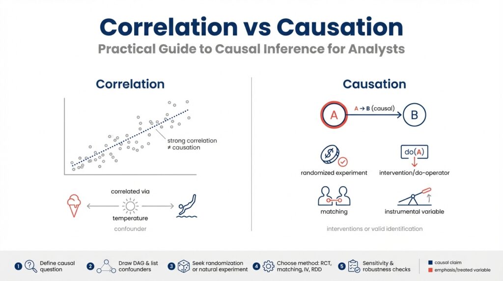
Correlation vs Causation Defined
Building on the foundation we established earlier, the difference between correlation and causation is the single most important distinction you’ll make when moving from descriptive analytics to causal inference. Correlation describes a statistical association: two variables move together more often than not, which you can quantify with measures like Pearson’s r, Spearman’s rho, or mutual information. These metrics tell you that a relationship exists in your dataset, but they do not tell you why that relationship exists or whether changing one variable will change the other.
Causation means one variable exerts a directional effect on another such that intervening on the cause changes the outcome. Causal language implies an underlying mechanism or process, and we formalize it as a causal effect—often represented in potential outcomes or structural causal models (SCMs). When you claim causation, you’re committing to a counterfactual statement: if you had intervened and set X to a different value, Y would have changed in a predictable way. This is why randomized experiments are the gold standard: randomization breaks systematic differences and lets us estimate that counterfactual reliably.
Knowing the distinction matters because your analysis choices and business actions depend on it. If you treat a correlation as causal, you may change product behavior, reallocate budget, or deploy models that produce no benefit—or cause harm—because the observed association was driven by something else. Conversely, if you ignore a true causal relationship, you might under-optimize interventions or miss a lever that would actually move metrics. So the practical question becomes: How do you tell whether a relationship is causal or coincidental?
Start by looking for common failure modes: confounding, reverse causation, and spurious correlation. Confounding occurs when a third variable influences both X and Y and creates an apparent association; for example, seasonality can make both sales and site visits rise simultaneously. Reverse causation is when the direction is flipped—higher sales might drive more marketing spend rather than the other way around. Spurious correlations can arise from data snooping, aggregation artifacts, or Simpson’s paradox where group-level trends reverse at the subgroup level. Run robustness checks, inspect time ordering, and stratify by plausible confounders to detect these problems.
In practice, use a pattern of evidence rather than a single test. Start with exploratory correlation analysis, then specify a causal question and map out assumptions using a DAG (directed acyclic graph). If you have an experiment, implement an A/B test and pre-register metrics; if not, consider quasi-experimental designs like difference-in-differences, regression discontinuity, or instrumental variables. You can also use matching or propensity-score adjustments as part of a design-based strategy. A small reproducible example in Python might look like this:
# naive: correlation
r = data['treatment'].corr(data['outcome'])
# adjusted: linear model controlling for confounders
import statsmodels.formula.api as smf
model = smf.ols('outcome ~ treatment + age + season', data=data).fit()
print(model.params['treatment'])
That snippet contrasts a raw correlation with a conditional estimate that controls for observable confounders; it doesn’t prove causality but illustrates the workflow analysts use to move from association to a causal estimate. Finally, treat causal claims as conditional on assumptions and data quality. If your business decision depends on an intervention, prioritize experimental or quasi-experimental validation, document your causal assumptions explicitly, and run sensitivity analyses to quantify how robust your conclusion is to hidden confounding.
Taken together, these practices turn vague associations into actionable insights. As we move into methods for identifying causal effects, we’ll apply these principles to concrete patterns you encounter in analytics pipelines and production experimentation systems.
Framing Causal Questions
Building on this foundation, the first practical step is to frame a precise causal question: this is where causal inference moves from an intellectual distinction into an actionable research plan. If you want to distinguish causation vs correlation in a way that supports decisions, you must be explicit about the intervention, the population, the time horizon, and the estimand (the numerical quantity you intend to estimate). How do you turn an observed association into a testable intervention that a product team or policy owner can act on? Asking that forces clarity about what data and design choices are appropriate.
Start by specifying the intervention and counterfactuals in plain language and a short mathematical form to avoid ambiguity. State what you would do differently: “set X to x (treatment) versus X to x’ (control) for members of population P over period T.” Then map that to a causal-effect target such as the average treatment effect E[Y(1) − Y(0)] or a conditional treatment effect E[Y(1) − Y(0) | Z = z] for a subgroup Z. This makes the causal effect concrete, tells you which variables you must measure, and guides whether randomized experiments, instrumental variables, or observational adjustments can answer the question.
Formalize your assumptions early and describe them visually with a DAG (directed acyclic graph). A DAG lets you encode background knowledge—time ordering, common causes, mediators, and potential colliders—and it clarifies which paths you must block to identify the causal effect. Define terms on first use: ignorability (no unmeasured confounding given controls), SUTVA (stable unit treatment value assumption, i.e., no interference across units), and consistency (the observed outcome under treatment equals the potential outcome for that treatment). When you write these assumptions down, you can test some empirically (balance checks, placebo outcomes) and acknowledge those you cannot.
Phrase your question in templates analysts can operationalize. One useful template is: “What is the effect of intervening to set X = 1 versus X = 0 on outcome Y in population P during time window T?” For example, “What is the effect of extending a free trial from 14 to 30 days on 90-day retention among new users who signed up in Q1?” That formulation immediately tells you the treatment definition, metric (90-day retention), cohort (new users), and cadence (Q1), which in turn informs sample sizing, randomization strata, and eligibility rules.
Let the framed question drive design choices: if you can randomize the intervention across the target population, run an experiment and pre-register the estimand and analysis plan; if not, search for quasi-experimental leverage that matches the intervention you care about. Difference-in-differences fits when rollout timing varies and pre-treatment trends are comparable; regression discontinuity works when assignment follows a clear threshold; instrumental variables help when you can find a source of exogenous variation that affects treatment but not the outcome directly. Describe why a chosen design maps to your estimand and which identifying assumptions it replaces or introduces.
Finally, translate the question into measurable specifications and robustness checks before you touch the data. Pre-specify the primary estimand, the metric definition, censoring rules, and subgroup analyses. Plan sensitivity analyses for unmeasured confounding and alternative model specifications, and state how you will interpret null or heterogeneous results. By framing causal questions this way, we keep the analysis honest, connected to decision-making, and ready for the methods—experimental or observational—that follow.
Experiments vs Observational Studies
When you move from spotting correlations to answering actionable questions, the most practical decision is whether to run randomized experiments or rely on observational studies. Randomized experiments (A/B tests and randomized controlled trials) should be your default whenever you can operationalize an intervention, because randomization severs systematic links between treatment and confounders and gives you a direct estimate of a causal effect. How do you decide when an A/B test is feasible, and when observational analysis is the more realistic route? We’ll walk through the trade-offs, practical checks, and patterns you can apply immediately in analytics work.
Randomized experiments give you a clear path to identification when you can assign treatment randomly. In a properly implemented A/B test, randomization balances both observed and unobserved confounders in expectation, which makes the difference-in-means a consistent estimator of the average treatment effect under SUTVA (no interference) and consistency. Practically, that means you should pre-register your estimand and analysis plan, stratify randomization on high-variance covariates if needed, and run balance checks before interpreting results. We recommend checking baseline covariates, running engagement sanity checks, and pre-specifying subgroup analyses; these operational steps reduce p-hacking and make your experiment credible to stakeholders.
Observational studies are what you use when you cannot randomize—because of cost, ethics, rollout constraints, or the nature of the question. An observational study uses naturally occurring variation and requires stronger assumptions to identify causal effects, such as ignorability (no unmeasured confounding) after conditioning on controls. In practice, that means combining design thinking with modeling: construct a DAG to surface plausible confounders, use matching or propensity-score weighting to improve balance on observables, and consider quasi-experimental designs like difference-in-differences, regression discontinuity, or instrumental variables when they map to your operational context. Observational work can answer questions experiments cannot (long-term effects, rare exposures, or historical policy evaluation), but you must be explicit about the assumptions that substitute for randomization.
Contrast the strengths and weaknesses in concrete terms to guide choices. Experiments excel at internal validity: they give unbiased estimates for the population and settings randomized, but they can be narrow (a short A/B test on new users) and expensive to run at scale. Observational studies often offer broader coverage, richer covariates, and longer horizons, but their validity depends on untestable assumptions and the quality of measured confounders. Moreover, some observational estimands target different causal quantities (for example, instrumental-variables estimates often recover a local average treatment effect rather than an average treatment effect for the whole population), so be careful when comparing experimental and observational point estimates.
Apply specific diagnostics and robustness checks to increase confidence no matter which path you choose. For experiments, run randomization inference and permutation tests, check for differential attrition, and monitor metrics for interference or saturation effects. For observational analyses, run placebo-outcome and placebo-treatment tests, inspect pre-treatment trends for DiD, and estimate sensitivity bounds for hidden confounding. We often run both: use observational signal to prioritize experiments, then use experiments to validate and quantify effects in a controlled setting, and finally use observational data to measure longer-term or broader impacts that are impractical to randomize.
Think about practical workflows rather than rigid hierarchies: when possible, design your analytics pipeline so experiments and observational studies complement one another. Use randomized experiments to establish causality and calibrate models; use observational studies to generalize those findings to production, to explore mechanisms, and to fill gaps experiments can’t cover. By treating causal inference as an engineering problem—define the estimand, state assumptions, choose the design that maps to your estimand, and run pre-specified diagnostics—you make defensible decisions that align technical rigor with product constraints.
Next, we’ll move from design choices to estimation and sensitivity techniques that let you quantify uncertainty and report credible causal estimates. For now, adopt the rule of thumb: randomize when you can; when you can’t, be deliberate about assumptions and use quasi-experimental or adjustment methods with thorough robustness checks to support your causal claims.
DAGs: Visualizing Causal Assumptions
Building on this foundation, start by translating your domain knowledge into a compact graphical language: a DAG (directed acyclic graph) that codifies the causal assumptions you cannot test with data alone. A directed acyclic graph is a set of nodes (variables) and directed edges (causal links) that enforce time ordering and forbid feedback loops; this visual shorthand forces you to state hypotheses about mechanisms before you fit models. How do you translate expert intuition and product rules into an analysis plan? By drawing the DAG first, you make explicit which variables are potential confounders, mediators, or colliders that will determine whether an observational estimate can be interpreted causally in your workflow.
A DAG’s basic elements are simple but powerful: a node represents a variable, an arrow indicates a directional effect, and a path is any sequence of arrows connecting two nodes. Define confounding on first use: a confounder is a common cause of both treatment and outcome that opens a non-causal path and biases naive associations. A collider is a variable influenced by two or more variables on different causal paths; conditioning on a collider creates spurious associations when none exist. By mapping these relationships visually we can apply rules—like the back-door criterion—to decide which variables to condition on and which to leave alone to obtain an unbiased estimate.
Use the DAG to derive a concrete adjustment set before you run regressions or matching. For example, if you’re estimating the effect of a pricing change on conversion and seasonality drives both traffic and willingness to pay, seasonality is a confounder you must adjust for. In contrast, if product exposure causes immediate engagement which then causes retention, that engagement is a mediator you should not adjust for when estimating the total causal effect. When a DAG highlights a collider—say, selection into a study based on both prior usage and treatment—you must avoid conditioning on that selection variable because doing so induces bias rather than removing it.
Operationalize DAGs in an analytics pipeline by treating them as living artifacts that guide variable selection, pre-registration, and sensitivity checks. Sketch the DAG with stakeholders to capture time ordering and plausible unmeasured confounders, then translate it into an adjustment strategy: list X variables to control in your regression, write down which variables are mediators to exclude, and specify any instrumental variables you plan to validate. We often encode the graph in simple code constructs (for example, graph.add_edge('seasonality','treatment') and graph.add_edge('seasonality','outcome')) and then document the adjustment set derived from the back-door paths so that analysts and engineers implement the same design.
Apply this approach to realistic scenarios you encounter: when you cannot randomize a free-trial extension, a DAG helps you separate marketing exposure (a confounder) from product usage (a mediator) and clarifies whether an instrument exists (for example, randomized eligibility thresholds). Why does this matter? Because the DAG tells you whether matching or propensity scores are appropriate, whether an IV is necessary, or whether a quasi-experimental design like difference-in-differences is a better fit given rollout timing. By encoding assumptions visually, you reduce post-hoc argument and make sensitivity analyses interpretable—stakeholders can see which unmeasured confounders would overturn your conclusion.
Finally, treat the DAG as the bridge from problem framing to estimation and sensitivity analysis: draw it before looking at outcome data, use it to pre-specify adjustment sets, and update it transparently as new domain knowledge emerges. When you follow this discipline, causal inference becomes a collaborative engineering step rather than an after-the-fact justification. In the next section we’ll apply these DAG-derived adjustment sets to concrete estimators and show how sensitivity bounds quantify the impact of potential unmeasured confounding.
Common Methods: Matching, IV, DiD
When you cannot run a randomized experiment, choosing the right quasi-experimental tool is the difference between a defensible causal claim and a misleading correlation. In causal inference we commonly reach for three families of methods—matching, instrumental variables, and difference-in-differences—because each trades different assumptions for identification. Which one you pick depends on what part of the causal problem you can credibly plausibly replace with data: observables, a valid instrument, or time-based exogenous variation. When should you use matching versus IV or DiD? Ask what assumptions you can defend in a DAG and what diagnostics you can run on your data.
Matching targets the problem of observable confounding by constructing a comparison group that looks like the treated group on measured covariates. The idea is straightforward: create treated and control units that are balanced on pre-treatment features so that differences in outcomes are more plausibly caused by the treatment. In practice you’ll implement exact matching, nearest-neighbor matching, caliper rules, or propensity-score matching and inspect balance with standardized mean differences and love plots; if balance fails, revise your specification or include richer covariates. Matching reduces model dependence and is especially useful when you believe unobserved confounding is weak but measured covariates explain treatment assignment well.
Instrumental variables (IV) replace the ignorability assumption with two alternative conditions: relevance (the instrument shifts treatment) and the exclusion restriction (the instrument affects the outcome only through treatment). IV is your tool when unmeasured confounders threaten matching or regression—provided you can find a credible instrument such as randomized encouragement, policy discontinuities, or plausibly exogenous supply shocks. Implementation typically follows two-stage least squares (2SLS): stage one predicts treatment from the instrument, stage two regresses outcome on predicted treatment. Watch for weak instruments (first-stage F-statistics below ~10 are a red flag) and remember IV estimates a Local Average Treatment Effect (LATE): the causal effect for compliers, not the whole population.
Difference-in-differences (DiD) exploits time variation in treatment assignment to difference out time-invariant confounding, estimating how treated and control groups diverge after an intervention. The central identifying assumption is parallel trends: absent treatment, treated and control would have followed the same trajectory. Practically, you implement DiD with a two-period estimator or panel fixed effects, plot event-study coefficients to check pre-trends, and consider staggered rollout adjustments when treatment timing varies across units. If pre-trends fail, DiD estimates are biased; if they hold, DiD gives intuitive, policy-relevant estimates, and event-study graphs give stakeholders a transparent visual diagnostic.
Each method brings strengths and caveats, so combine them when it improves credibility. Use matching to improve overlap and balance before running DiD or IV; run placebo outcomes and placebo dates to test for spurious signals; and estimate sensitivity bounds to quantify how strong an unmeasured confounder would need to be to overturn your result. For example, match new users on registration cohort and baseline engagement, then run a DiD on retention before and after a staged feature rollout—this reduces reliance on functional-form assumptions and clarifies the estimand for stakeholders.
In practice, adopt a reproducible workflow: sketch a DAG to justify which assumptions you’re replacing, pick the method that maps to those assumptions, pre-specify the estimand and diagnostics (balance, first-stage strength, pre-trends), and report robustness checks alongside point estimates. By treating matching, instrumental variables, and difference-in-differences as complementary tools rather than competitors, we produce more credible causal inference and clearer guidance for product and policy decisions. Next, we’ll use these diagnostics to choose estimators and quantify uncertainty so you can present findings with appropriate caveats and actionable recommendations.
Practical Workflow and Diagnostics
Building on our earlier framing and DAG work, the practical task is to turn assumptions into an operational causal inference pipeline that surfaces failures early and quantifies uncertainty. Start by declaring the estimand, the population, and the hypothesized back‑door paths in a short README so everyone agrees on what we’re estimating and why. This early specification anchors downstream diagnostics and makes the analysis auditable; it also helps you automate checks and document which assumptions—ignorability, SUTVA, exclusion—are critical for interpretation.
A repeatable workflow reduces ad‑hoc choices and prevents confirmation bias. Organize the pipeline into discrete stages: pre‑analysis data validation, design selection (experiment or observational), estimation with pre‑specified models, diagnostics and sensitivity analysis, and production monitoring. How do you structure an analysis pipeline that surfaces assumption failures early? Put simple, testable gates between stages: only proceed to estimation if balance and overlap checks pass, only promote a result to stakeholders after robustness checks meet pre‑defined thresholds, and log every decision for reproducibility.
Start with rigorous data validation and pre‑treatment checks before you touch outcomes. Verify time ordering, check for duplicated or imputed IDs, inspect missingness patterns, and create cohort tables that show flow from eligibility to treatment. For observational designs, evaluate common support by plotting propensity‑score overlap and compute standardized mean differences for baseline covariates; for experiments, run balance tables and randomization inference. Visual diagnostics—histograms, love plots, and event‑study graphs—often reveal problems that summary statistics hide.
Select and implement the design that maps to your DAG and business constraints, then instrument the process for diagnostics. If you can randomize, pre‑register the estimand, stratify randomization on high‑variance covariates, and embed checks for differential attrition and interference. If you must use observational tools, operationalize matching, IV, or DiD as dictated by the DAG and pre‑specify balance metrics, first‑stage strength rules (watch F < 10), and pre‑trend windows for DiD. Implement these choices in code templates so colleagues reproduce the same design choices.
Run layered diagnostics and robustness checks to quantify how fragile your causal claims are. Execute placebo outcomes and placebo dates, permutation tests, and estimate sensitivity bounds that report how strong an unmeasured confounder would need to be to change the conclusion. Report heterogeneous effects with pre‑specified subgroup analyses and correct for multiple comparisons when appropriate. For example, match new users on registration cohort and baseline activity, then run a DiD with event‑study coefficients plus Rosenbaum or E‑value style bounds to communicate both point estimates and fragility.
Make reproducibility and monitoring part of the workflow, not an afterthought. Version your DAGs and analysis scripts in the same repo, produce a small human‑readable pre‑analysis plan, and run CI checks that fail the pipeline when balance, overlap, or first‑stage thresholds are violated. When an experiment or policy rolls to production, deploy lightweight monitoring to detect treatment drift, changing composition, or metric divergence so you can re‑run diagnostics and update estimates as context evolves.
When we treat causal inference as an engineering workflow—define the estimand, lock the design, run pre‑specified diagnostics, and quantify sensitivity—we create results stakeholders can act on with measured confidence. The next step is to choose estimators and formal sensitivity techniques that map to these diagnostics; by following this pipeline, we make interpretation transparent and keep causal claims tethered to explicit, testable assumptions.