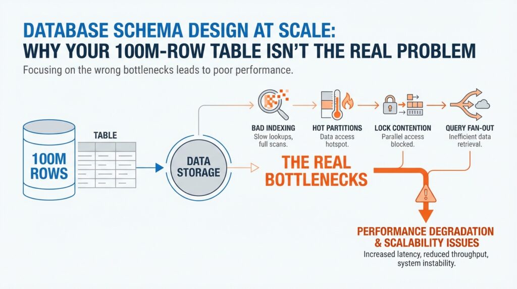
Find the Real Bottleneck
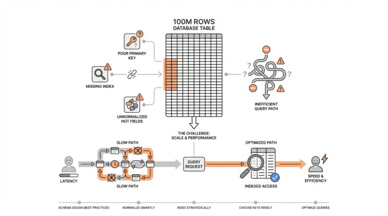
Building on this foundation, the first thing we want to do is stop staring at the row count and start watching the path the database takes to answer a question. A 100M-row table can feel intimidating, but the real slowdown usually lives somewhere else: in the query plan, the planner’s estimate of how many rows it expects, or the extra work caused by a bad access path. Think of it like driving across a city. The city can be huge, but your trip gets slow because of the route, traffic, and red lights—not because the map has too many streets. How do you tell whether the pain comes from the table itself or from the route the database chose? Start there, because database schema design at scale is really about finding the slowest step, not the largest object.
Once that idea clicks, we can look at the query itself like a recipe with too many moving parts. EXPLAIN shows the query plan, which is the database’s step-by-step strategy for fetching data, and EXPLAIN ANALYZE goes one step further by actually running the query and showing the real row counts and runtime at each step. That matters because a plan that looks efficient on paper can still be wrong in practice if the planner’s statistics are stale or incomplete. In PostgreSQL, ANALYZE refreshes the statistics the planner uses, and the documentation recommends it after major data changes so the optimizer can choose a better plan. In other words, if the database is guessing wrong, the bottleneck may be misinformed decision-making rather than raw table size.
With the query plan in hand, we can separate a slow statement from a crowded system. pg_stat_statements is a statistics view that records execution and planning behavior for queries, which helps you find the statements that consume the most time across the whole workload instead of chasing one-off slow requests. If the database is not merely slow but stuck, pg_locks shows outstanding locks, and the lock-monitoring docs explain that it can help you spot contention that is blocking progress. This is where a lot of people discover the surprise: the table was never the bottleneck at all. The real issue was that one long transaction, one hot row, or one overloaded write path was making everyone else wait in line.
Now that we know where to look, schema design at scale becomes much less mysterious. A large table can still perform well when the database can use the right index, and PostgreSQL’s default index type is B-tree, which works well for common comparisons like equality and range filters. Partial indexes can also help when only a subset of rows matters, because they avoid indexing values you rarely search for. So when a query feels slow, we should ask a sharper question: is the database scanning too much data, sorting too much data, waiting on locks, or choosing the wrong index entirely? That question keeps us focused on the bottleneck we can actually fix instead of the table size we can only fear.
Model Access Patterns First
Building on this foundation, we stop asking how big the table is and start asking how the data is read. How do you design a schema when one part of the app wants a single customer by ID, another wants the last 30 days of activity, and a third wants a queue of work items in order? The answer is to model access patterns first: write down the exact questions your system asks most often, because database schema design at scale lives or dies by those repeatable paths, not by raw row count. PostgreSQL’s index and partitioning docs both point in the same direction: the best structure depends on the kinds of lookups, ranges, and hot subsets you need to serve.
Once we name those paths, the table starts to split into familiar shapes. A point lookup feels like checking one address in a contact list, while a date range feels like flipping to a month in a planner; the first wants a fast exact match, and the second wants an order the database can walk without wandering. PostgreSQL’s default B-tree index is built for equality and range comparisons, which is why it fits so many common read patterns. When your query asks for the “next” or “between” rows, that shape matters more than the table’s total size.
Now the interesting part: some data is hot, and most data is not. If your app mostly touches a small slice—open orders, active subscriptions, unbilled invoices—you do not want every row carrying the same indexing burden. Partial indexes let you index only the subset that matters, which makes the index smaller and the matching queries cheaper to serve; partitioning goes one step further by grouping rows so heavily used partitions can stay compact and memory-friendly. In PostgreSQL, partition pruning can even skip partitions entirely during planning or execution when the query makes that possible.
Access patterns also show up in the way columns travel together. If you almost always filter by customer_id and status at the same time, the planner can misread that pair as two unrelated conditions unless it has better statistics to work with. PostgreSQL’s extended statistics can capture dependencies, most-common-value lists, and multicolumn behavior so the optimizer has a clearer picture of the data distribution. This is one of those quiet wins in database schema design: you are not only shaping storage, you are teaching the planner how your workload behaves.
With that mindset, schema decisions become a conversation about traffic, not vanity. You begin by asking which read path must feel instant, which slice of data stays hottest, and which columns tend to travel together; only then do indexes, partitions, and constraints start to make sense. That is why access-pattern-driven design feels so powerful: once we know the road, we can build the road instead of hoping the table size will somehow explain the slowdown.
Choose Better Partition Keys
Building on this foundation, choosing better partition keys is where the table starts to feel less like a single massive object and more like a set of smaller, manageable neighborhoods. A partition key is the column, or sometimes the combination of columns, that decides where each row lives. Think of it like sorting mail before delivery: if you already know the street, the post office can send the envelope down the right route without checking every address in the city. That same idea is at the heart of database schema design at scale, because the right partition key can turn a broad scan into a narrow, focused search.
How do you choose a partition key that helps instead of hurts? We start by looking at the questions your application asks most often, then we ask which field appears in those questions consistently. If most requests look up recent events, a time-based key such as created_at may fit well. If the workload centers on tenant-specific data, tenant_id may be the better boundary. The key point is that the partition key should line up with the way the data is read, not with how it happens to be stored today.
This is where people sometimes reach for the wrong signal. A partition key should not be chosen because it feels important or because it is unique; it should be chosen because it groups related rows in a way the database can use. A customer ID sounds appealing, but if each customer has only a few rows, you can end up with too many tiny partitions and more overhead than benefit. On the other hand, a date column can be powerful when your queries naturally ask for “this week,” “this month,” or “the last 30 days,” because the database can skip whole chunks of data that fall outside that window.
Stability matters just as much as selectivity. If the value in your partition key changes often, the row has to move, and that creates extra work that feels invisible until the system grows. That is why partitioning usually works best with values that stay put, such as when the row was created, which tenant owns it, or which region it belongs to. In database schema design at scale, we want boundaries that support the workload without forcing the data to keep changing neighborhoods.
Now that we understand the shape of a good partition key, we can talk about balance. A useful partition key spreads rows in a way that avoids one hot partition becoming a traffic jam while the others stay quiet. If one partition receives nearly all the writes, you have not really solved the bottleneck; you have only moved it to a smaller room. The goal is a partitioning strategy that keeps each slice useful on its own, while still making it easy for the database to prune away the slices you do not need.
There is also a practical maintenance benefit hiding here. Smaller partitions are easier to vacuum, archive, back up, and drop when old data no longer matters, which is why partitioning often becomes attractive long after the first performance problem appears. That does not mean every large table needs it, though. If your queries rarely include the partition key, or if the data does not naturally group into a few clear access paths, partitioning can add complexity without much payoff. In that case, a well-chosen index may be the better answer.
So the real test is whether the partition key matches the way the table is actually used. When the key lines up with your hottest filters, your most common time windows, or your most important tenant boundaries, the database gets to work with smaller, more relevant pieces of data. And once that starts making sense, the next question becomes even more interesting: how do you decide how many partitions you really need, and how fine-grained should those boundaries be?
Prevent Hot Partitions
Building on this foundation, the next problem is not the table’s size but one partition becoming the place where every request lands. If your reads and writes keep funneling into a single slice, the rest of the table can be perfectly healthy and the system still feels stuck. How do you keep one partition from turning into a traffic jam? You start by treating database schema design at scale as a routing problem, because PostgreSQL’s partitioning only pays off when typical queries let the planner prune most partitions and focus on a small number of relevant ones.
Think of it like a grocery store with several checkout lanes, except one lane ends up serving almost everyone. Adding more lanes helps only if shoppers are actually spread across them. That is the practical lesson we can infer from PostgreSQL’s guidance: the planner performs best when it can eliminate most partitions, and performance gets worse as more partitions remain after pruning. In other words, a “hot partition” is really a routing mistake in disguise.
So what does that mean in practice? We choose the partition key based on the queries that show up most often, not on the column that feels the most important in the abstract. PostgreSQL’s best-practices section says the best choice is often the column or columns that most commonly appear in WHERE clauses, because those are the filters the planner can use to prune unneeded partitions. If your workload is dominated by recent activity, a time-based key can line up with those lookups; if it is dominated by tenant-specific traffic, a tenant key may be the better boundary.
Now we need to be careful, because a good-looking key can still create a bad outcome if one value dominates the workload. If one customer, region, or status owns most of the inserts and updates, that partition becomes the busy sidewalk while the others stay quiet. PostgreSQL even warns us to think ahead about future growth, and it suggests using HASH partitioning with a reasonable number of partitions when a simple list-style layout might become awkward over time. Taking that advice together, the goal is not “one partition per thing”; the goal is to spread traffic in a way that stays balanced as the system grows.
This is where hot-partition prevention and index design meet. A partition that carries the hottest rows should also stay lean, because PostgreSQL notes that partition pruning depends on partition bounds rather than indexes, and it also says an index is most helpful when a query scans only a small part of a partition. Partial indexes help here too: PostgreSQL describes them as indexes over a subset of a table, especially useful for avoiding common values and reducing update overhead. That means we can keep the busiest slice narrower instead of making every row pay the same indexing cost.
There is also a quiet trap in going too far. PostgreSQL says the planner can handle partition hierarchies with up to a few thousand partitions fairly well only when queries prune all but a small number of them, and it warns that planning time and memory use rise as more partitions survive pruning. It also cautions that too many partitions increase both planning and execution overhead, while too few can leave indexes oversized and data locality poor. So the real balancing act is not “more partitions versus fewer partitions,” but “enough partitions to spread heat, not so many that we create a new bottleneck in the planner.”
Before we go further, it helps to test the shape of the traffic instead of guessing. PostgreSQL recommends using EXPLAIN to see whether pruning is happening, and EXPLAIN ANALYZE to compare the planner’s estimates with real execution. It also notes that simulations of the intended workload are often beneficial when choosing a partitioning strategy. That is exactly how we avoid hot partitions in practice: we test the real query patterns, watch which slices stay busy, and adjust the boundaries before the heat becomes a production problem.
Add Indexes Strategically
Building on this foundation, we can start treating indexes like tools with a job, not decorations on a table. A 100M-row table does not need more indexes by default; it needs the right index for the questions your application asks over and over. How do you know which one deserves the space? We begin with the shape of the lookup, because PostgreSQL’s default B-tree index fits the most common situations, especially equality, range, and ordered searches.
The first strategic choice is often a composite, or multicolumn, index, which is an index built on more than one column. This is where order matters: PostgreSQL says a multicolumn B-tree index works best when the leading, leftmost columns carry the most useful constraints, because equality on those columns narrows the scan first, and an inequality on the first non-equality column can narrow it further. That means an index on (customer_id, status) behaves very differently from one on (status, customer_id), even if the same columns appear in the query. In other words, strategic indexing starts by matching the index order to the way your most important filters arrive.
Now that we have the search path in mind, we can ask whether the database really needs to visit the table at all. If a query repeatedly reads a small set of columns, a covering index can carry those extra columns as payload through the INCLUDE clause, which makes an index-only scan possible when the data is visible and the query only needs columns stored in the index. That can be a big win on read-heavy tables, but PostgreSQL also warns us to be conservative: included columns bloat the index, wide payload columns can make inserts fail if the tuple gets too large, and the payoff is limited when the table changes constantly. So the trick is not “include everything”; it is “include only what turns a common read into a cheap walk through the index.”
Partial indexes are the next lever, and they are especially useful when only a slice of the table matters. PostgreSQL defines a partial index as an index over a subset of rows, and one major reason to use it is to avoid indexing common values that the planner would not want to use anyway. That shrinks the index and also reduces update work, because rows outside the predicate do not need index maintenance. But partial indexing only works when the query conditions line up with the predicate, and PostgreSQL is strict here: if the planner cannot prove that the query implies the predicate, it will not use the index, especially for parameterized queries.
This is where strategic indexing becomes a story about restraint. Every index is another structure the database must store and maintain, so the goal is not to scatter them everywhere but to create a few that pay rent every day. PostgreSQL even notes that B-tree indexes on tables with many inserts or updates can benefit from lower fillfactor settings when you build them, and CREATE INDEX CONCURRENTLY lets you build an index without blocking concurrent writes. That tells us something important: when write traffic is heavy, we should think not only about whether an index helps reads, but also about how much extra work it adds to the write path.
So when you are deciding whether to add an index, ask the same question a careful mechanic would ask before replacing a part: what exactly is the failure mode? If the query needs a better leftmost key order, build a composite index. If it reads the same columns again and again, consider a covering index. If only a small subset of rows matters, reach for a partial index. And if you are not sure, let EXPLAIN ANALYZE show you whether the plan is actually using the shortcut you built, because it reports real row counts and real execution time, not guesses.
Partition for Growth
Building on this foundation, partitioning becomes less about chasing speed and more about making growth manageable. When a table keeps expanding, the real pain often shows up in the routines around it: vacuuming takes longer, backfills become riskier, old data is harder to archive, and even a routine cleanup can feel like opening a giant suitcase on a crowded train. That is why partitioning matters in database schema design at scale. It gives you smaller pieces to work with, so the table can keep growing without forcing every operation to become a full-table event.
What happens when your data outgrows a single maintenance routine? That is the question to keep in mind as we look at growth-friendly layouts. A partitioned table lets the database treat each slice as its own manageable unit, which means you can work on recent data, cold data, and expired data in different ways. For example, an events table often needs fast access to the last few days, while older events mostly sit in the background. Instead of keeping all rows in one crowded room, partitioning lets us separate the active space from the archive space, which makes the system easier to operate as it scales.
This is where the long-term value starts to show up. Smaller partitions are easier to vacuum, analyze, back up, and drop, so the database can spend less effort on data that no longer matters to the business. That matters because growth is not only about serving more reads and writes; it is also about keeping the house in order while the furniture keeps multiplying. In database schema design at scale, that operational breathing room is often the difference between a system that ages gracefully and one that becomes fragile every time you need to clean it up.
At the same time, partitioning works best when the data naturally arrives in waves. If your workload has a clear time pattern, like orders by day or logs by month, a time-based partition key can line up with the way people actually ask questions of the data. If your system is multi-tenant, a tenant-based partition key may help isolate traffic and keep one customer’s activity from dominating every operation. The main idea is to match the partitioning strategy to the shape of the workload, not to force the workload to fit a neat design you chose in advance.
That said, growth can expose a hidden trap: too many partitions can make the database work harder, not easier. Each extra partition adds planning overhead, and if most queries cannot prune away the irrelevant ones, the database has to consider more paths than you intended. So the goal is not to create a partition for every possible category or every tiny slice of data. The goal is to create enough separation to make pruning effective, while keeping the layout simple enough that the planner can still move quickly through it.
This is also where partitioning and indexing start to cooperate. Once the data is split into smaller chunks, each partition can carry only the indexes it truly needs, which keeps maintenance lighter and makes the hot working set easier to fit in memory. That is a subtle but powerful shift in database schema design at scale: instead of asking one giant table to serve every access pattern, we let each partition specialize a little. A recent-data partition can stay lean and fast, while older partitions can be indexed differently or even treated as mostly read-only.
So when we think about partitioning for growth, we are really planning for change. We are giving the table room to expand without turning every maintenance job into a crisis, and we are creating boundaries that help the database spend its energy where it matters most. If the partition key matches the real workload, the partitions stay balanced, and the pruning stays effective, growth feels a lot less like a threat. It starts to look like a system with enough structure to keep moving forward, even as the row count keeps climbing.