Assess Workload Patterns (learn.microsoft.com)
Before we split a database into pieces, we need to watch how the traffic actually moves. That is the heart of sharding: the best design depends less on the size of the data alone and more on the workload patterns behind it—how often you read, how often you write, which records get hit together, and whether most requests cluster around a few users, regions, or time periods. How do you know whether sharding will help your database? Start by tracing the requests that arrive most often and asking which ones must stay together to avoid extra hops.
Once that picture becomes clearer, the next question is whether your shard key can follow the shape of those requests. A shard key is the attribute that tells the system where a row belongs, and Microsoft recommends choosing one that is immutable, high-cardinality, and aligned with your dominant query patterns so most requests land on a single shard. That matters because queries that stay inside one shard are faster and simpler, while cross-shard queries add latency, extra resource use, and more moving parts. In other words, if your everyday path looks like “find one customer and their orders,” the data model should help that conversation stay local instead of sending it across town.
Now that we understand the shape of the questions, we can look at the shape of the answers. Some workloads naturally behave like a single lane road, where range-based access works well because related items arrive in sequence and are often read together; others behave more like a crowd, where hash-based sharding helps spread load and reduce hotspots. A hotspot is a shard that receives a disproportionate amount of traffic, and Microsoft calls out monotonically increasing values, low-cardinality fields, and frequently changing attributes as common ways to create one. So if your workload keeps asking for “the newest” or “the most active” records, that is a clue to look for a distribution method that does not dump all the pressure onto one shard.
Tenant behavior and geography also tell a story worth listening to. In a multitenant system, one noisy tenant can dominate shared resources, so the source recommends thinking about whether highly volatile tenants should live in separate shards to protect everyone else’s performance. Geography matters too: if users in the same region mostly read and write the same data, placing that data nearby can lower latency and support residency requirements, but it can also create uneven load if one region is much busier than the others. That is why workload assessment is not only about data volume; it is about where the pressure comes from and whether it arrives evenly or in bursts.
We also need to check which kinds of questions the application asks most often. If the dominant pattern is cross-entity joins, multi-entity transactions, or full-dataset aggregation, sharding can become a poor fit because those operations become expensive once data is split apart. Microsoft’s guidance is to keep most operations scoped to a single shard, denormalize related data when it is commonly queried together, and use secondary indexes or fan-out queries only when you truly need them. That is the quiet lesson here: assess workload patterns first, because the cleanest sharding design is the one that matches how your system already behaves, not the one that forces every request to become a distributed puzzle.
Design Access-Friendly Schema (postgresql.org)
Building on this foundation, an access-friendly schema is about making the database feel natural to the questions your application asks most often. A schema is the blueprint of your data: which tables exist, how they connect, and where each piece of information lives. When you design it well, PostgreSQL can find rows with fewer detours, and your queries behave more like a straight path than a maze. How do you design a schema that stays fast when real users start clicking, searching, and filtering?
The first step is to group data by how it is read, not only by what it is. Think of it like organizing a kitchen: ingredients used together should be close at hand, even if they could be stored in separate cabinets. In a database, that often means placing closely related information in tables that join cleanly, and keeping the most common lookup fields easy to reach. This is where access patterns matter again, because a schema that looks elegant on paper can still feel slow if every request has to jump across several tables.
Now we can introduce two ideas that often tug in opposite directions: normalization and denormalization. Normalization means splitting data into smaller tables so each fact lives in one place, which reduces duplication and makes updates safer. Denormalization means keeping some repeated or combined data together so reads need fewer joins, which can speed up common queries. The art of an access-friendly schema is choosing the right balance, so you protect data quality without forcing every request to assemble the same puzzle pieces over and over.
This is also where indexes earn their keep. An index is a data structure that helps the database locate rows faster, much like a book’s index helps you jump to a topic without reading every page. In PostgreSQL, good indexes usually follow your most frequent search conditions, sort orders, and join columns, because those are the places where the engine spends the most time looking. If your application often asks for orders by customer, for example, a customer identifier in both the orders table and its index can make that path much smoother.
Primary keys and foreign keys deserve the same careful attention. A primary key is the main identifier for a row, and a foreign key is a column that points to a row in another table, like an order pointing back to its customer. When these keys line up with real-world relationships, joins become easier to reason about and easier for the database to optimize. If the keys are awkward, oversized, or chosen without thinking about lookup patterns, the schema can become harder to query even before you reach sharding.
Let us make this concrete. Suppose most of your application shows a customer’s recent orders, their shipping status, and the products inside each order. An access-friendly schema would keep the customer record stable, store orders with a clear customer reference, and place the most searched columns where PostgreSQL can index them efficiently. You might still separate line items into their own table, but you would design that split with the expectation that reads will frequently travel from customer to order to item in the same direction.
The real goal is not to flatten everything or to split everything apart. It is to shape the schema so the database can answer common questions with the fewest surprises. When you keep the hottest paths short, choose indexes that match those paths, and avoid forcing routine reads into expensive joins, your schema starts to work with the workload instead of against it. That same idea becomes even more important when we move from table design into the next layer of performance tuning.
Choose Horizontal Scaling (docs.aws.amazon.com)
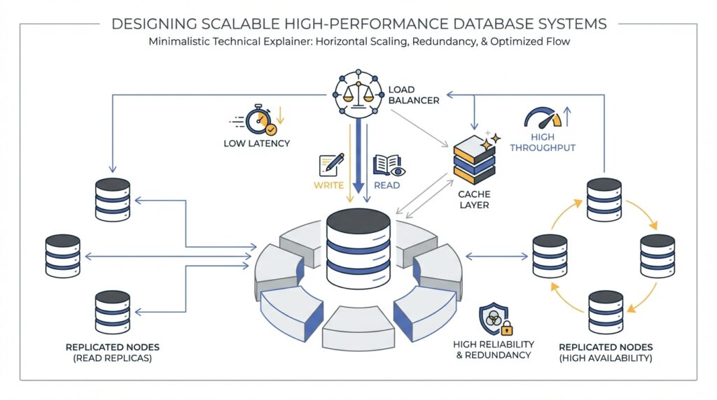
Building on the workload map we just drew, horizontal scaling is the moment where the database stops feeling like one crowded counter and starts feeling like a row of open lanes. In Amazon DocumentDB, elastic clusters use hash-based sharding, which spreads data across multiple shards instead of forcing growth into a single box, and each shard has a writer plus optional read replicas. That matters because the service separates compute from storage, so you can add capacity by spreading work across more shards rather than only making one node bigger. How do you know this is the right move? You choose it when your goal is to widen throughput for reads and writes while keeping the storage layer distributed behind the scenes.
The next decision is the shard key, the field that tells the cluster where each document belongs. Think of it like choosing the aisle label in a warehouse: if the label spreads items evenly, workers move fast; if one label attracts everything, the room clogs. AWS recommends an evenly distributed hash key, using that key in read, update, and delete requests so you avoid scatter-gather queries, and steering clear of nested shard keys for those same paths. For batch work, setting ordered to false lets shards work in parallel, which keeps one slow part from holding everyone else back.
This is where horizontal scaling either feels graceful or turns awkward. It shines when traffic can be spread across many shards and when you watch for hot keys, which are values that attract too much traffic and create a hotspot on one shard. AWS suggests tracking per-shard CPU, free memory, cursors, and document activity, because a large peak-to-average gap tells you the load is uneven even when the cluster looks healthy at first glance. In practice, that means you are not only asking, ‘Can I add more shards?’ but also, ‘Will my data actually use them evenly?’
Scaling also has a rhythm, and it pays to respect it. DocumentDB notes that scaling operations can cause brief intermittent database and network errors, so the safest move is to avoid peak hours and use a maintenance window when you can. If you need a faster adjustment, changing vCPUs per shard is usually the preferred knob because it completes more quickly and with a shorter disruption window; when you can anticipate growth, adding shards earlier gives you more room to expand later. That is the difference between widening the road before rush hour and trying to move traffic while it is already packed.
The cleanest horizontal scaling plan is the one that matches your earlier workload and schema decisions. If most routine reads and writes stay inside one shard, the cluster can spread pressure without turning every request into a cross-shard puzzle; if your most active collections are unsharded, AWS recommends keeping heavily used ones on different databases because unsharded collections in the same database are co-located on the same shard. So as you move forward, keep the goal in mind: make the cluster feel wider, not messier. That is what turns horizontal scaling from a rescue tactic into a design choice.
Optimize Index Strategy (postgresql.org)
Building on the schema work we just did, index strategy is where the database starts learning which roads deserve a fast lane. An index is a separate structure that helps PostgreSQL find rows faster, but it also adds overhead to inserts, updates, and deletes, so every index should earn its place. That is why the question is not, “How many indexes can we add?” but “Which few indexes will pay back the most during real queries?”
How do you choose those winners? Start with the questions your application asks most often, then match the index to that shape. In PostgreSQL, a B-tree index is the workhorse for exact matches, ranges, and sorted output, and it can even satisfy an ORDER BY without a separate sort step when the order lines up. That makes it a strong first choice for columns that filter, join, or sort the same way over and over, especially when you only need a small slice of the table.
Now let us add a little structure to that idea. A multicolumn index is like a library card catalog organized by more than one label, such as customer_id and created_at together. PostgreSQL can use a multicolumn B-tree index with any subset of its columns, but it works best when the leading, leftmost columns appear in the query; later columns help most when earlier ones are already constrained. That is why a composite index should usually reflect the way your users search, not the order that happens to look neat on paper, and why very wide indexes are rarely worth the extra space and write cost.
Sometimes the smartest index is the one that ignores most of the table. A partial index covers only rows that satisfy a predicate, so it is perfect when one small slice of data gets most of the attention, such as open orders, active accounts, or unbilled records. Because the index is smaller, it is faster to scan and cheaper to maintain, but it only helps when the query’s WHERE clause clearly implies the same predicate; parameterized clauses can miss that match. In other words, partial indexes are a sharp tool, not a universal shortcut.
Here is where things get even more practical. If your searches use transformed data, an expression index can store the transformed value itself, such as lower(email) for case-insensitive lookup. And if a frequent query needs only a few columns, a covering index can include those extra columns so PostgreSQL can answer the request with an index-only scan, which avoids fetching the table row at all when the index type supports it and every needed column is already in the index. Think of it like packing the exact ingredients you need into one lunchbox instead of walking back to the pantry mid-recipe.
There is one more habit that keeps index strategy honest: test it against real data. PostgreSQL can combine multiple indexes with bitmap scans when no single index fits the query well, so two focused indexes may be better than one oversized composite index in some cases. The planner also relies on up-to-date statistics, which is why PostgreSQL recommends running ANALYZE and checking EXPLAIN or EXPLAIN ANALYZE before deciding an index is a real win. If an index never shows up in the workload, drop it and let the write path breathe again.
The calmest PostgreSQL index strategy is the one that mirrors the workload, keeps the hottest paths short, and leaves everything else alone. When we choose indexes this way, the database feels less like a maze and more like a well-marked route map, which is exactly what a growing system needs.
Add Replication and Caching (docs.aws.amazon.com)
Building on the workload map we already drew, replication and caching are the two levers that keep a busy database from feeling crowded. Replication gives you more places to answer the same question, while caching keeps the most recently used data close to the engine so it does not have to travel far for every read. How do you make that happen without turning your cluster into a tangle of moving parts? In Amazon DocumentDB, the answer starts with a primary instance for writes and one or more replica instances for read scale, then continues with a cache that helps hot data stay ready for the next request.
The first part of the story is replication itself. A single Amazon DocumentDB cluster can have one primary instance and up to 15 replica instances, and you can spread them across Availability Zones in the same Region. The primary handles both reads and writes, while replicas are read-only, which means they can absorb read traffic without competing with writes on the writer. Reads from replicas are eventually consistent, and AWS says replica lag is usually very small, often under 50 milliseconds, though heavy write activity can increase it.
Once the replicas exist, the next question is where your application sends its reads. This is where the driver, meaning the client library your app uses to talk to the database, becomes important. AWS recommends connecting as a replica set through the cluster endpoint and using built-in read preferences, such as secondaryPreferred, so the driver can send reads to replicas and keep writes on the primary. That setup also helps the client discover the cluster automatically as replicas are added or removed, and it avoids the fragility of forcing every read to go only to secondary, which can fail if no replica is available.
Caching is the quiet partner in this setup. Amazon DocumentDB keeps its page cache in a separate process, so the cache can survive independently of the database process and remain in memory after a restart. In practical terms, that means the buffer pool, a block of memory that holds recently used data pages, can wake up already warmed instead of starting from cold. AWS also exposes cache statistics through collection stats, including hit and miss ratios, so you can see whether your workload is finding data in memory or falling back to disk more often than you want.
So what does that mean in practice? If you see a low BufferCacheHitRatio, high ReadIOPS, or a primary that is nearing CPU limits, your working set is probably stretching beyond what one instance can keep hot. AWS recommends watching CPUUtilization, DatabaseConnections, and BufferCacheHitRatio, because those signals tell you when reads are crowding the primary or the cache is not carrying enough of the load. In that situation, scaling up can be the right first move because a larger instance gives you a bigger buffer cache per database instance before you start spreading traffic across more nodes.
For especially read-heavy workloads, AWS also points to NVMe-backed instances as another cache-friendly option. These instances use local SSD storage as a second-tier cache, while the in-memory buffer cache stays the first tier, and AWS says that setup can help when the dataset is larger than memory and read latency starts to climb. That is a useful mental model: replicas give you more read hands, while better caching helps each hand work faster. If your application spends most of its time rereading recent documents, those two improvements often work best together.
When we put replication and caching side by side, the design becomes easier to picture. Writes still flow through one primary, read traffic fans out to replicas, and hot data stays closer to memory so the same customer profile, order history, or dashboard metric does not have to be fetched from slower storage over and over again. If you need strict read-after-write behavior for a particular request, keep that path on the primary; if the read can tolerate a tiny delay, let the replicas carry it. That balance is what turns Amazon DocumentDB replication and caching from a safety feature into a performance strategy.
Monitor Plans and Statistics (postgresql.org)
Building on the index work we just did, the next question is whether PostgreSQL is actually taking the route we expected. You can choose a strong index and still get a slow query if the planner believes the data looks different from reality, which is why monitoring query plans and statistics matters so much. Think of it like checking a map after a long drive: the route may look right on paper, but we still need to see how the trip really unfolded. How do you tell? By looking at the plan the planner chose and the statistics it used to make that choice.
The first tool in that conversation is EXPLAIN. It shows the query plan as a tree of plan nodes, where the lower nodes usually scan tables and the upper nodes handle joins, sorting, or aggregation. Each line includes cost estimates, and those costs are what the planner tries to minimize when it chooses a plan. In other words, EXPLAIN is the planner’s sketch of the route, not the trip itself.
Once we have that sketch, EXPLAIN ANALYZE lets us compare it with reality. With this option, PostgreSQL actually runs the query and then reports the true row counts and true execution time for each node alongside the estimates. That makes it much easier to spot where a plan looks good on paper but drifts in practice, which is exactly the kind of mismatch that can make a previously healthy query start to feel heavy. If you are trying to answer, “Why is this query slower than I expected?”, this is usually the best place to start.
But those plans are only as good as the statistics behind them, so ANALYZE becomes the quiet partner in the story. PostgreSQL stores the results in the pg_statistic catalog, and the planner uses them to decide which execution plan is most efficient. The database can run this automatically through autovacuum when tables are loaded or changed, but after major data shifts it is wise to refresh the statistics manually so the planner is not working with an old snapshot of the table. ANALYZE also uses a random sample for large tables, which keeps it fast but means its results are approximate and can change slightly from one run to the next.
That approximation is usually fine, but it becomes interesting when estimated rows and actual rows disagree by a wide margin. When that happens, the planner may be missing a skewed value distribution, or a column may need a richer statistics target so PostgreSQL can build a better picture of the data. The statistics gathered by ANALYZE commonly include most-common values and a histogram of the distribution, and you can raise or lower that level of detail with default_statistics_target or per-column settings. So if a hot column keeps confusing the planner, you do not have to guess blindly; you can give it better evidence.
A practical monitoring habit is to start broad, then narrow the mystery. First, run EXPLAIN to see which plan PostgreSQL prefers, then use EXPLAIN ANALYZE on a safe test query or in a controlled environment to compare estimates against real behavior. If the gap is large, look at the columns used in filters, joins, and sorts, because those are the places where stale or thin statistics often cause the planner to misread the workload. For tooling and automated checks, EXPLAIN can also emit machine-readable formats such as XML, JSON, or YAML, which makes it easier to track plan changes over time.
The bigger lesson is that plans and statistics are a feedback loop, not a one-time setup step. Every time your data distribution changes, your indexes, joins, and filters are telling PostgreSQL a new story, and ANALYZE is how you help the planner hear it clearly. Once you can read that story, the next tuning decision becomes much less mysterious.