MAE overview and objectives
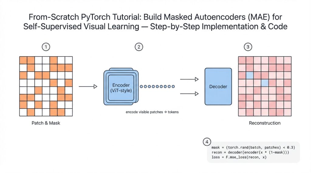
Masked Autoencoder (MAE) is a self-supervised learning approach that trains a model to reconstruct missing parts of an image from partial context, forcing the encoder to learn rich visual representations without labels. By masking a large fraction of input patches and asking the model to predict the original pixels for those masked patches, MAE converts unlabeled images into an effective pretext task for representation learning. Why does masking help self-supervised visual learning? Because it creates a prediction problem that requires both local texture understanding and global scene context, so the encoder must capture hierarchical features useful for downstream tasks.
Building on this foundation, the core architecture follows an encoder-decoder pattern tuned for efficiency: a vision transformer (ViT) encoder consumes only the unmasked patch tokens, and a lightweight decoder reconstructs pixel values for the masked patches. We assume you’re familiar with patch embedding (splitting an image into non-overlapping patches and projecting them), so the key twist is heavy masking—typical configurations mask 70–80% of patches—so the encoder computes far fewer token representations per image. The decoder has lower capacity and operates on full token sets (visible + mask placeholders) to reconstruct pixels, which incentivizes placing most representational burden in the encoder while keeping compute budget predictable.
The principal objective during pretraining is reconstruction: minimize an image-space loss (commonly mean squared error) between the predicted and original pixel values for masked patches, but only over masked regions so the model cannot trivially copy visible inputs. That pretext loss produces intermediate encoder embeddings we can freeze or fine-tune: linear probing evaluates how linearly separable classes are from frozen features, while full fine-tuning adapts the encoder to downstream tasks like classification, detection, or segmentation. Practically, you’ll pretrain on large unlabeled corpora (e.g., ImageNet or domain-specific imagery) and then fine-tune with standard supervised objectives—MAE representations often yield faster convergence and superior transfer performance compared with training from scratch.
There are concrete engineering benefits you can exploit. Because the encoder only processes visible tokens, wall-clock throughput for encoder forward passes increases proportionally to the masking ratio—this makes MAE computationally attractive for large-scale pretraining. The reconstruction target also encourages robustness to occlusion, which is valuable in real-world scenarios such as aerial/satellite imagery where clouds hide areas, or medical imaging where lesions occupy small regions and labels are sparse. In practice, teams use MAE to pretrain models on unlabeled institutional datasets and reduce labeled-data requirements for downstream tasks, improving sample efficiency and reducing annotation cost.
Design choices matter and change behavior in predictable ways: masking ratio, patch size, decoder depth, reconstruction target, and data augmentation each trade off representation quality, compute, and reconstruction fidelity. Start experiments with 75% masking, 16×16 patch size for ImageNet-scale inputs, and a shallow decoder (1–4 transformer blocks), then sweep mask ratios and decoder widths based on downstream metrics. Using pixel-wise MSE is a simple default, but perceptual losses or frequency-weighted losses can prioritize high-frequency details if you care about texture reconstruction. Finally, pay attention to augmentation: heavy geometric or color augmentations can harm pixel reconstruction, so prefer milder transforms during pretraining or apply augmentation only to visible patches.
Next we’ll translate these principles into an actionable PyTorch implementation: you’ll implement patchify/unpatchify utilities, deterministic masking and random masking schedules, an encoder that accepts variable subset tokens, a decoder that reconstructs masked patches, and a training loop that computes the masked MSE loss and logs both reconstruction and downstream-proxy metrics. Along the way we’ll instrument throughput and GPU memory usage so you can tune masking for your hardware, and show how to export pretrained weights for downstream fine-tuning pipelines.
Prerequisites and environment setup
Building on this foundation, the first practical step is getting an environment where MAE training is reliable and repeatable: a GPU-backed PyTorch setup, reproducible Python environment, and fast data pipeline so we can iterate on masking ratios and decoder depth without hardware surprises. If you’re preparing for large-scale self-supervised pretraining, prioritize a workstation or cluster node with a modern NVIDIA GPU and 16+ GB of device memory for comfortable batch sizes; smaller experiments can run on 8 GB cards with aggressive gradient accumulation. You should expect to allocate tens to hundreds of gigabytes of disk for datasets and checkpoints when using ImageNet-scale corpora, and ensure your OS has up-to-date NVIDIA drivers and CUDA runtime compatible with your chosen PyTorch wheel.
Start by isolating dependencies in a virtual environment to avoid version drift between experiments. Create a Conda or venv environment pinned to a stable Python 3.9–3.11 interpreter, then install PyTorch and core libraries such as torchvision, timm (for model utilities), numpy, and an experiment tracker you prefer (for example, Weights & Biases). Keep dependency installation declarative in a requirements.txt or environment.yml so you can rebuild the exact environment later; this pays off when you want to reproduce a checkpoint or share weights with colleagues. We recommend installing PyTorch from the official selector appropriate to your CUDA runtime rather than guessing wheel tags; that prevents mismatches between the driver, toolkit, and installed binaries.
How do you verify CUDA and PyTorch see the GPU? Run a short Python check inside the environment to confirm availability and device names before launching long jobs. For example:
import torch
print('cuda available:', torch.cuda.is_available())
if torch.cuda.is_available():
    print('device:', torch.cuda.get_device_name(0))
    print('count:', torch.cuda.device_count())
A green light here avoids wasted training runs and helps you debug driver, CUDA, or container issues early. For deterministic experiments, set a fixed seed for torch, numpy, and random, and be aware that full determinism with CuDNN can impact performance; choose reproducibility or speed based on the experiment’s objective.
Organize your data for high-throughput patch extraction and random masking. For prototyping, a simple folder of images works, but for production-scale pretraining prefer fast formats like WebDataset, LMDB, or sharded TFRecords equivalents to avoid filesystem bottlenecks. Decide on input resolution (commonly 224) and patch size (we typically use 16×16 for ImageNet-scale inputs) before building the data loader so augmentation pipelines and tensor shapes remain consistent. Since heavy pixel reconstruction is sensitive to aggressive color or geometric transforms, keep pretraining augmentations conservative and perform any heavy augmentations only during downstream fine-tuning.
Plan for distributed training and mixed precision from the start so scaling later is straightforward. Use PyTorch Distributed Data Parallel (DDP) with an NCCL backend and launch with torchrun/torch.distributed to run across multiple GPUs or nodes; prefer per-GPU batch sizes small enough to fit memory and scale total effective batch size via gradient accumulation. Enable AMP (automatic mixed precision) via torch.cuda.amp to reduce memory footprint and improve throughput on modern GPUs; this is particularly effective for MAE because the encoder processes fewer tokens per image, shifting the compute balance toward the decoder and optimizer state.
Finally, instrument logging, checkpointing, and experiment metadata before training long pretraining runs. Save periodic checkpoint files containing encoder weights and optimizer state, track training and masked-MSE loss curves via your tracker, and store the exact environment.yml or pip freeze output alongside code. With a reproducible environment, verified GPU access, sharded datasets, and a distributed/mixed-precision launch pattern, we can confidently move to implementing patchify/unpatchify, deterministic masking, and the encoder-decoder components that will form the core of the masked autoencoder training loop.
Data preprocessing and patchify
Building on this foundation, the first practical bottleneck you hit when training a masked autoencoder at scale is how you convert raw images into the token stream the ViT encoder expects. Data preprocessing determines effective token count, numeric stability, and how expensive per-step masking will be, so allocate attention to resizing, normalization, and the patch extraction pipeline early in your experiment. Patchify is more than a convenience function: it’s the bridge between image pixels and transformer tokens, and small mistakes here cascade into wrong shapes, mismatched reconstruction targets, or wasted GPU cycles.
Start preprocessing by fixing your input resolution and color normalization strategy; this decision sets the patch grid and total patches per image. How do you choose patch size and resolution? Pick a patch size that balances spatial granularity and token count—16×16 on 224×224 gives 14×14 patches, while 8×8 multiplies tokens and memory cost. During preprocessing, resize with a deterministic interpolation (e.g., bicubic) and optionally pad to a multiple of the patch size to avoid partial patches; store image tensors as float32 (or float16 when using AMP) and apply the same mean/std normalization you’ll use during fine-tuning to keep statistics consistent.
Implement patch extraction with tensor operations rather than Python loops to avoid CPU-GPU transfer overhead. The typical PyTorch pattern reshapes and permutes to produce patches in channel-major order, then flattens spatial patches into vectors for a linear projection. For example:
# x: [B, C, H, W]
patch_size = 16
x = x.reshape(B, C, H//patch_size, patch_size, W//patch_size, patch_size)
# move patch dims together -> [B, C, Hn, Wn, ph, pw]
x = x.permute(0, 2, 4, 1, 3, 5).reshape(B, Hn*Wn, C*patch_size*patch_size)
# linear projection -> patch embeddings
emb = linear_proj(x)  # [B, N_patches, embed_dim]
Pay careful attention to memory layout: use contiguous tensors before reshape when necessary, and prefer fused projection kernels (Conv2d with stride=patch_size is an alternative) when memory bandwidth is the bottleneck. Keep an unpatchify inverse handy for the decoder: reconstruct patch vectors, reshape back to [B, C, ph, pw, Hn, Wn], permute, and reshape to [B, C, H, W] for loss computation. This symmetrical mapping guarantees pixel-aligned MSE losses and simplifies masking bookkeeping.
Masking decisions must align with your patch indices and the loss mask you compute during preprocessing. Generate per-sample mask indices with a reproducible RNG (torch.Generator seeded per-sample or per-worker) and collapse masked patch positions into an indexing tensor you pass to the encoder/decoder. For deterministic experiments, save the RNG seed alongside checkpoints so you can exactly replay a masked batch. Decide whether to mask uniformly at random, with block masks, or using low-frequency heuristics depending on the data modality—medical scans or satellite imagery often benefit from structured masks that reflect occlusion patterns.
Operationally, decide whether to patchify on the fly in the data loader or precompute and store patches. On-the-fly patchify with num_workers>0 and pinned memory keeps storage manageable and allows dynamic augmentations, while precomputed patches (LMDB/WebDataset) buy throughput at the cost of storage and preprocessing time. If you choose on-the-fly, optimize the DataLoader with sufficient workers, use tensor transformations (not PIL) inside collate, and profile CPU vs GPU time—patchify is cheap per image but scales with dataset size and can become the critical path.
Real-world imagery introduces edge cases: non-square images, variable resolutions, and modalities with different channel counts. For these, either resample to a canonical size before patchify or support adaptive patch grids with dynamic positional embeddings. Overlapping patches or multi-scale patching can improve reconstruction for fine textures, but they increase token counts and complexity; reserve those strategies for downstream tasks like segmentation where spatial fidelity matters.
Taking this concept further, a robust preprocessing and patchify pipeline reduces debugging time and gives predictable token budgets for MAE training. With a reproducible patch extraction, deterministic masking, and a clear mapping from patch indices to pixels, we can move on to implementing the encoder that consumes sparse tokens and the decoder that reconstructs masked patches.
Model: ViT encoder and decoder
Building on this foundation, we now map the MAE architecture into concrete encoder and decoder components you can implement and tune. The ViT encoder should be thought of as a heavy feature extractor that only touches visible patch embeddings, which is the primary efficiency win in a masked autoencoder. Start by projecting patchified pixel vectors into an embedding space (for example, a linear layer or a Conv2d with stride=patch_size), add a learnable cls token if you need classification downstream, and apply positional embeddings before token selection. By front-loading these steps you keep the encoder input compact and predictable while preserving spatial alignment for later reconstruction and downstream probing.
The encoder consumes a variable-length sequence of visible tokens selected by mask indices rather than the full N patches; this is how we reduce compute proportional to (1 – mask_ratio). How do you design the encoder so it only processes visible tokens efficiently? Use boolean masking or index-based gather to select embeddings per sample (torch.gather or advanced indexing), then run those through a stack of transformer blocks (LayerNorm, Multi-Head Self-Attention, MLP) sized for representation quality—typical ImageNet-scale setups use 12–24 blocks and embed_dim 512–1024. Keep normalization placement consistent (pre-norm is common) and ensure you maintain deterministic per-sample ordering so the decoder can place encoded tokens back into their original spatial slots.
The decoder is intentionally lightweight and operates on the full token set (visible encoded tokens + mask placeholders) to predict pixel-level targets only for masked patches. Implement a single learnable mask token and insert it at masked positions; then add positional embeddings that cover all N patches so the decoder sees absolute spatial information for both visible and masked slots. Use a small transformer for the decoder (1–4 blocks, lower embed_dim and fewer heads) followed by a simple predictor head that projects decoder outputs for masked positions back to patch-sized pixel vectors. Finally, unpatchify those predicted vectors to reconstruct image patches and compute the reconstruction loss (commonly MSE) only over the masked patch pixels to avoid trivial copying.
Design choices here dictate where capacity and compute live: put representational weight in the ViT encoder and keep the decoder narrow so training remains fast while preserving reconstruction quality. For example, increasing encoder depth improves downstream linear-probing performance more reliably than deepening the decoder, while widening the decoder can help pixel fidelity if texture reconstruction is your priority. Decide whether to share positional embeddings between encoder and decoder—sharing reduces parameters and can stabilize alignment, while separate embeddings let the decoder learn finer reconstruction priors. Also choose whether the mask token is a learned vector or a structured initializer (Gaussian noise or scaled visible mean); learned mask tokens are effective in practice and simple to implement.
From an implementation and performance standpoint, pay attention to efficient token selection and memory layout. Batch-level variable-length sequences can be handled with padded tensors plus attention masks, or by processing concatenated visible tokens per-batch and reconstructing per-sample positions with index maps; the latter often gives better throughput on GPU by avoiding wasted compute on padding. Use torch.cuda.amp to enable mixed precision, gradient checkpointing for very deep encoders, and DDP for multi-GPU scaling; these engineering choices let you maintain aggressive mask ratios without running out of memory. When computing loss, compute the reconstruction MSE only on the masked patch indices and accumulate metrics that separately track masked loss and visible-similarity to spot leakage.
Here’s a compact end-to-end mental flow you can code quickly: patchify -> linear projection -> add pos -> select visible indices -> encoder transformer stack -> scatter encoded tokens back into full N slots with mask tokens for masked indices -> add pos -> decoder transformer stack -> predictor head -> unpatchify -> masked MSE. With concrete shapes in mind (e.g., 224×224, patch=16 → N=196; mask 75% → 49 visible tokens), you can benchmark encoder-only throughput and tune decoder capacity accordingly. In the next section we’ll translate this module-level design into PyTorch classes and walk through the exact tensor operations and indexing patterns to implement the encoder and decoder efficiently.
Masking strategy and loss
Building on this foundation, the choices you make for how to mask patches and compute the loss determine both the learning signal and the computational trade-offs for MAE pretraining. A deliberate masking strategy influences which features the encoder must encode: high random masking forces global context learning, block or structured masking emphasizes local completion, and semantic or saliency-aware masking targets class-relevant regions. How do you pick a mask ratio that balances compute and representation quality? We typically treat the masking ratio as a primary hyperparameter to sweep (common starting point: 0.7–0.8) and evaluate both masked reconstruction loss and downstream linear-probe accuracy to find the sweet spot for your dataset and budget. Keywords: masking strategy, MAE, masked autoencoder.
Think about mask topology next: uniform random masks are the default because they maximize ambiguity per patch and scale well across domains, but they can under-represent contiguous occlusions found in real-world data like clouds in satellite imagery or surgical occlusions in medical scans. Block masks (contiguous windows) increase the decoder’s need for long-range reasoning and improve robustness to extended occluders, while stratified masks (mix of large blocks and single patches) let you train both fine texture and global structure recovery. For domain-specific work, design masks that reflect the real occlusion patterns you expect downstream; this aligns the pretext task with practical invariances and often improves transfer.
Implement masking deterministically per-sample and reproducibly per-epoch so you can replay batches for debugging and curriculum experiments. Use a per-worker torch.Generator seeded from a global RNG to ensure parallel DataLoader workers produce stable masks across runs, and store mask indices alongside checkpoints if you need exact replay. Consider mask schedules: a fixed high mask ratio is simple, but linearly increasing masking across epochs or randomly annealing helps the encoder gradually build context priors; we often start with lower masking for early stability then ramp to 75% over the first 10–20 epochs when training from scratch.
Loss formulation matters more than most engineers expect. The canonical approach is masked MSE computed only on masked patch pixels, which prevents trivial copying and focuses supervision on the reconstruction target. In PyTorch you can compute this efficiently by indexing masked patch positions and applying reduction over pixels per patch, then normalizing by the number of masked pixels to keep losses comparable across mask ratios. Here’s a focused pattern you can adapt:
# pred: [B, N_masked, P*P*C], target: same shape, mask_count: scalar per-batch
err = (pred - target).pow(2)
per_patch = err.mean(dim=-1)          # mean over pixels in patch
loss = per_patch.mean()               # mean over masked patches
# or normalize explicitly: loss = per_patch.sum() / mask_count
Normalize the loss by masked pixel count or masked patch count so that different mask ratios and batch sizes yield comparable magnitudes; this is critical when you monitor training curves or tune learning rates. Also track both masked-only and full-image reconstruction metrics: masked-only loss shows pretext learning, while full-image similarity (or a perceptual metric) surfaces whether the model learned useful global structure versus overfitting to local textures.
Beyond L2, choose robust or perceptual objectives when your downstream goals require texture fidelity or semantic alignment. L1/Charbonnier losses reduce sensitivity to outliers and can produce sharper patches, while perceptual losses computed on intermediate layers of a frozen CNN or a frequency-weighted MSE emphasize high-frequency detail and texture. For most representation-learning objectives focused on classification transfer, standard masked MSE delivers strong linear-probe performance; opt for perceptual or frequency losses only when you explicitly need better visual fidelity for downstream tasks like segmentation or synthesis.
From an operational perspective, log and instrument carefully: report masked MSE, unmasked similarity, per-channel errors, and a small qualitative grid of reconstructed patches each validation step to catch mode collapse or color shifts early. When you scale training with mixed precision, compute the loss in float32 before backward to avoid numerical issues with small masked regions. These practices make the masking strategy and reconstruction loss reliable levers you can tune to push MAE representations from basic contextual completion to transferable, robust features for your downstream workloads.
Training loop and fine-tuning
Building on this foundation, the heart of a successful MAE workflow is a disciplined training loop that maximizes GPU throughput while preserving reproducibility and signal quality. Start each iteration by loading a batch, applying the patchify path you already implemented, and generating deterministic masks (seed per-worker) so experiments are replayable. In PyTorch you’ll combine mixed precision (torch.cuda.amp) with per-GPU batch sizes and optional gradient accumulation to hit target effective batch sizes without OOMs. Treat the training loop as an orchestration layer: data → patchify → mask → encoder → scatter → decoder → masked-loss → backward → step, and instrument each handoff for timing and correctness.
Implement the core loop so the forward/backward path is clear and debuggable; here’s a compact pattern you can adapt and expand. Use autocast for the forward pass and scale the loss before backward to keep numerical stability when using float16. Make optimizer steps only after unscaling gradients and optionally apply gradient clipping for very deep encoders. Example PyTorch skeleton:
scaler = torch.cuda.amp.GradScaler()
for batch in loader:
    patches = patchify(batch)
    masks, vis_idx = sample_masks(patches)
    with torch.cuda.amp.autocast():
        enc_out = encoder(patches[:, vis_idx])
        dec_out = decoder(scatter(enc_out, masks))
        loss = masked_mse(dec_out, targets, masks)
    scaler.scale(loss).backward()
    if accumulate_step_reached:
        scaler.unscale_(optimizer)
        torch.nn.utils.clip_grad_norm_(model.parameters(), max_norm)
        scaler.step(optimizer); scaler.update(); optimizer.zero_grad()
Choice of optimizer and learning-rate schedule materially affects convergence in MAE pretraining. We typically use AdamW with standard betas (0.9, 0.95) and decoupled weight decay; exclude biases and LayerNorm parameters from decay to preserve normalization dynamics. Scale the base learning rate with the effective batch size (linear scaling rule) and use a short linear warmup (e.g., 2–10 epochs) before a cosine decay—this stabilizes early reconstruction learning. How do you schedule learning rate and warmup for MAE pretraining? Start conservative when training from scratch, then increase the rate when fine-tuning on large labeled sets, and track masked-MSE and validation linear-probe accuracy to validate choices.
Checkpointing, metrics, and validation should be first-class citizens in your loop rather than afterthoughts. Save checkpoints that include encoder state_dict, optimizer, scaler, current epoch, RNG seeds, and optionally the last mask RNG so you can exactly replay a failing batch; this saves debugging hours. Validate periodically on a held-out set, computing masked-only MSE and logging small qualitative grids of reconstructed patches to spot color shifts or collapse. In distributed runs use per-worker logging with rank-0 aggregation for visual artifacts and keep throughput, memory usage, and per-step latency as primary operational metrics alongside loss curves.
When you shift from pretraining to fine-tuning, the training loop and hyperparameters should change deliberately rather than by default. Start with linear probing (freeze encoder, train a new head) to assess representation quality quickly, then run progressive fine-tuning: unfreeze top transformer blocks first or apply discriminative learning rates (lower lr for pretrained encoder, higher lr for new head). Increase augmentation strength and regularization during fine-tuning—stronger color jitter, RandAugment, and mixup often help classification—because reconstruction pretraining relied on conservative augmentations. In practice, reduce weight decay for the head, use a slightly higher learning rate for classification, and enable AMP and DDP as in pretraining to keep experiments comparable.
Finally, operationalize common debugging and scaling patterns so you can iterate fast. If reconstructions collapse to blur, check mask generation, per-sample normalization, and whether the decoder is too powerful relative to the encoder; conversely, if linear-probe performance lags, prioritize deeper/wider encoder capacity rather than increasing decoder depth. Automate resume-from-checkpoint and reproducibility checks, sweep mask ratio and decoder width with low-overhead short runs, and keep your training loop implementation modular so you can swap loss variants (L1, perceptual) without invasive changes. With these practices in place, you’ll convert a robust MAE training loop into a predictable fine-tuning pipeline that reliably transfers learned features to downstream tasks.