What is a CNN?
A convolutional neural network is a specialized deep-learning model built to process images and other grid-like data. It replaces the dense, fully connected layers of classic neural nets with convolutional layers that learn small filter kernels (e.g., 3×3) and slide them across the image to produce feature maps. Each filter performs a dot product over its receptive field, so the same set of weights is reused at every spatial location (weight sharing), which greatly reduces parameters and gives the network translation sensitivity and efficiency.
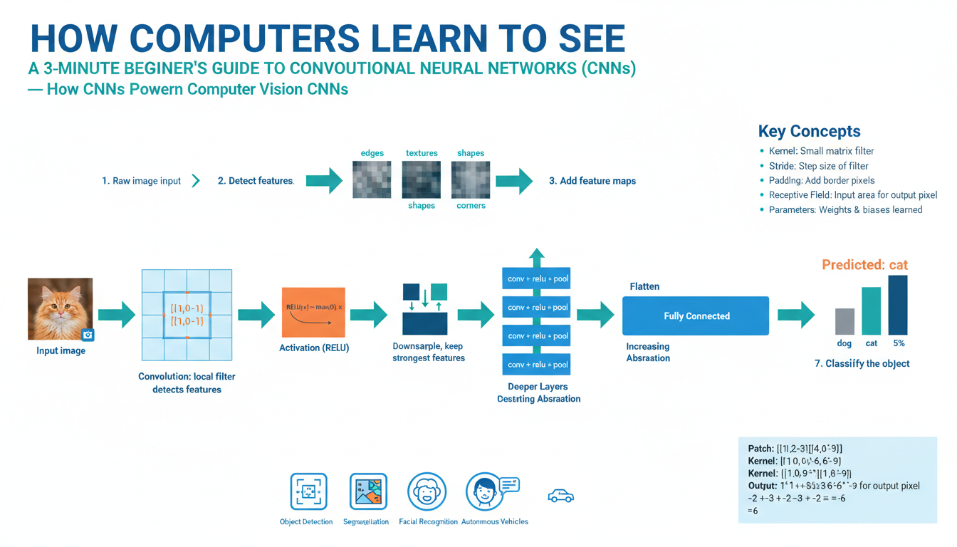
Layers typically alternate between convolution, a nonlinear activation (commonly ReLU), and optional pooling or downsampling. Early convolutional layers capture low-level patterns like edges and corners; deeper layers combine those into textures, parts, and object-level concepts. After many convolutional stages, a classifier (fully connected layers or global pooling + a final linear layer) maps learned features to outputs such as class probabilities. Training optimizes filter weights by backpropagating a loss (e.g., cross-entropy) using gradient-based optimizers.
This architecture excels at tasks where spatial hierarchies matter: image classification, object detection, semantic segmentation, and feature extraction for transfer learning. Its core strengths are local connectivity, hierarchical feature learning, and parameter efficiency—qualities that let computers “see” and generalize visual patterns from pixels to high-level concepts.
Images as Grid Data
Digital images are simply numeric grids: a height-by-width lattice where each cell stores one or more channel values (e.g., RGB). In practice an image is represented as a tensor with shape H × W × C (for example 224 × 224 × 3), where each entry is an intensity or normalized float. That grid structure encodes spatial relationships—nearby pixels tend to correlate—so local patterns like edges, corners, and textures appear as small, reusable motifs across the image.
Convolutional models exploit this by operating on local neighborhoods: a convolutional kernel (e.g., 3×3) has weights for a small receptive field and is applied repeatedly across every spatial location. For color images a single kernel has shape kH × kW × C and collapses the channel dimension to produce one feature map; multiple kernels produce multiple channels of features. Weight sharing (the same kernel at all positions) gives translation equivariance and drastically reduces parameters compared with fully connected layers.
Because the input is a grid, common operations are spatial: strides move the kernel, padding preserves border information, and pooling or strided convolutions reduce H and W while increasing receptive field. Thinking of images as structured tensors—not unordered vectors—explains why convolutions are both efficient and effective at extracting hierarchical visual features from pixels to objects.
How Convolution Works
A convolutional filter is a small, learnable matrix (a kernel) that scans an image and computes a dot product at every spatial location to produce a feature map. For a grayscale patch the operation is elementwise multiplication of the kernel and the patch followed by summation; for a color image a single kernel has shape kH × kW × C (for example 3×3×3) and collapses the channel dimension, producing one channel of output. Applying the same kernel across all positions is called weight sharing and gives the model translation equivariance and far fewer parameters than a fully connected layer.
Stride and padding control how the kernel moves and how borders are handled: a larger stride downsamples spatial resolution, while padding preserves edge information. A layer typically applies many kernels in parallel so the output becomes a stack of feature maps, each responding to a different learned pattern (edges, textures, color blobs). Nonlinear activations (e.g., ReLU) follow to introduce complexity, and pooling or strided convolutions increase the effective receptive field so deeper units see larger regions and can represent parts and objects.
During training the network adjusts kernel weights by backpropagating a loss; kernels that detect useful motifs are strengthened. In short, convolution turns local, repeated image motifs into compact, hierarchical feature representations that power modern computer vision.
Activation and Nonlinearity
Convolutional layers compute linear responses; the elementwise nonlinear transform that follows is what lets a network learn complex, hierarchical functions instead of collapsing to a single linear mapping. Activations are applied independently to every value in a feature map (so shapes like H×W×C stay the same) and are typically placed immediately after the convolution and before any pooling or downsampling.
Common choices balance simplicity, gradient flow, and numerical behavior. The rectified linear unit ReLU(x)=max(0,x) is the default in modern CNNs because it is cheap, introduces sparsity, and mitigates vanishing gradients. Variants like Leaky ReLU keep a small slope for negative inputs to avoid “dead” units. Sigmoid and tanh once dominated but tend to saturate for large magnitudes, causing vanishing gradients—useful in some output layers or small networks but less common in deep convolutional stacks. For multiclass classification the final layer often uses softmax to produce probabilities.
Activation choice affects learning speed and stability: piecewise-linear functions enable effective gradient propagation, while saturating functions require careful initialization and lower learning rates. In practice, combine a robust activation with normalization (e.g., batch norm) and appropriate initialization to get fast, stable training and richer feature representations.
Pooling and Downsampling
Convolutional networks routinely shrink spatial maps between stages to cut computation, grow the receptive field, and emphasize higher‑level patterns. A common, cheap way is a small window (for example 2×2) slid with stride 2: max pooling keeps the largest activation in each window (good for preserving strong responses and adding small-shift robustness), while average pooling smooths features. Global pooling collapses each channel to a single number and often replaces large fully connected layers to reduce parameters and overfitting.
Downsampling can be implemented as strided convolution instead of fixed pooling; because kernels are learned, strided convs often keep more task‑relevant information. When precise spatial localization matters (detection, segmentation), avoid aggressive downsampling or recover detail with encoder–decoder structures and skip connections. Aliasing is another practical concern: applying a simple low‑pass (blur) before reducing resolution or using anti‑aliased pooling improves shift‑equivariance. Alternatives and refinements include overlapping/learnable pooling, stochastic pooling, and dilated convolutions (which enlarge receptive field without decreasing spatial size). In practice, 2×2 max pooling or a small-stride convolution is a solid default for classification, with global average pooling before the final classifier; choose learnable or anti‑aliased strategies when preserving spatial information is critical.
Training and Backpropagation
Training a convolutional network means turning prediction errors into weight changes. A loss (e.g., cross‑entropy for classification) measures how far the network’s output is from the target; backpropagation applies the chain rule to compute gradients of that loss with respect to every parameter by propagating error signals backward through convolution, activation, pooling, and normalization layers. For convolutions, gradients accumulate over all spatial positions where a kernel was applied, so a single filter’s update reflects many local patches.
Parameters are updated by an optimizer that uses those gradients: the simplest rule is gradient descent (w ← w − lr·∇w), while practical training uses variants like SGD with momentum or Adam to speed convergence and stabilize noisy mini‑batch estimates. Mini‑batch training balances gradient signal and compute; use a validation set to monitor generalization and trigger early stopping or learning‑rate changes. Good defaults: He/kaiming initialization with ReLU, batch normalization to steady gradient flow, and a moderate learning rate with a scheduler (step, cosine, or reduce‑on‑plateau).
Watch for practical failure modes: vanishing/exploding gradients in very deep nets (mitigate with residual connections, normalization, careful init), overfitting (use weight decay, dropout, and data augmentation), and unstable updates (use gradient clipping or lower learning rate). For quick prototyping, Adam helps; for best final accuracy, many practitioners switch to SGD with momentum and tuned schedules. Regularly visualize training/validation loss and sample predictions—these simple checks catch label bugs, data leaks, and capacity mismatches early.