Why indexing matters
Building on this foundation, database indexing is the practical lever you pull when queries start costing seconds instead of milliseconds. A well-designed B-Tree index reduces disk I/O and CPU by turning full-table scans into targeted lookups, directly improving query performance for reads, range scans, and ordered results. If you’ve ever asked “Why is this query slow on production?” the answer is often a missing or misused index. We’ll treat index selection as both a performance tool and a capacity-management decision rather than a black box.
An index is a data structure that maps key values to row locations so the database can avoid scanning unrelated rows; in relational systems that structure is most commonly a B-Tree. The important benefits are reduced latency for point lookups and efficient range queries, which translate into fewer page reads and smaller working sets in memory. Two terms you should know are selectivity (how many distinct values a column has) and cardinality (the count of distinct items); high selectivity columns usually yield the biggest gains when indexed. These trade-offs matter because indexes change the cost profile of queries and the storage footprint of your database.
Indexes bring costs as well as benefits: every insert, update, or delete must maintain the index structure, adding write amplification, storage use, and potential contention. How do you decide which columns to index? Favor columns that are used frequently in WHERE, JOIN, ORDER BY, or GROUP BY clauses and that have decent selectivity; avoid indexing low-selectivity boolean flags unless combined with other columns. Consider composite indexes when queries filter on multiple columns—order matters, so make the leftmost column the one you filter on most often. When write throughput is critical, balance the number of indexes against the performance hit of maintaining them.
Concrete examples help. In an e-commerce orders table where queries often look up recent orders by user, create an index like CREATE INDEX idx_orders_userid_created_at ON orders (user_id, created_at DESC); to support both the lookup and the ordering without extra sorting. If you have a hotspot query that selects status, COUNT(*) FROM orders WHERE created_at > ? GROUP BY status, a partial index or an index on (created_at, status) can turn an expensive aggregation into a fast index-only scan. Covering indexes—which include all columns a query reads—can avoid the row lookup entirely and eliminate random I/O; for instance, including total_amount in the index lets SELECT created_at, total_amount FROM orders WHERE user_id = ? be served from the index alone.
Why is the B-Tree the dominant choice for these patterns? B-Trees are height-balanced, keep nodes densely packed to minimize disk seeks, and support logarithmic-time searches with very fast leaf-level sequential reads for ranges. That combination makes them excellent for ordered retrievals and range scans compared with hash indexes, which are great for exact matches but ineffective for range queries. In practice you’ll see the difference as index seeks (targeted traversal) versus index scans (reading contiguous leaves); seeks are low-latency, scans are efficient when the result set is large but will still touch more pages than a selective seek.
Measure and iterate: use EXPLAIN/EXPLAIN ANALYZE to validate that queries use the intended index and to quantify the difference in logical reads and execution time. Monitor index bloat, fragmentation, and statistics—set appropriate fillfactor where you expect heavy updates to avoid frequent page splits. If an index is unused, drop it; if an index accelerates a hot path, keep it and consider tuning its columns or creating a partial/covering variant. Next, we’ll dissect B-Tree internals—node layout, page splits, and balancing—to understand exactly why these behaviors appear and how to tune them for predictable query performance.
B-Tree fundamentals
Building on this foundation, we now examine how the data is physically organized inside a B-Tree so you can reason about latency, write amplification, and tuning trade-offs. The most important takeaway up front is that a B-Tree packs many keys and pointers into fixed-size pages (or nodes), which keeps tree height very low and minimizes random I/O. Understanding node layout—what lives in internal nodes versus leaf nodes—and the arithmetic that determines branching factor (fanout) gives you the levers to control performance under real workloads.
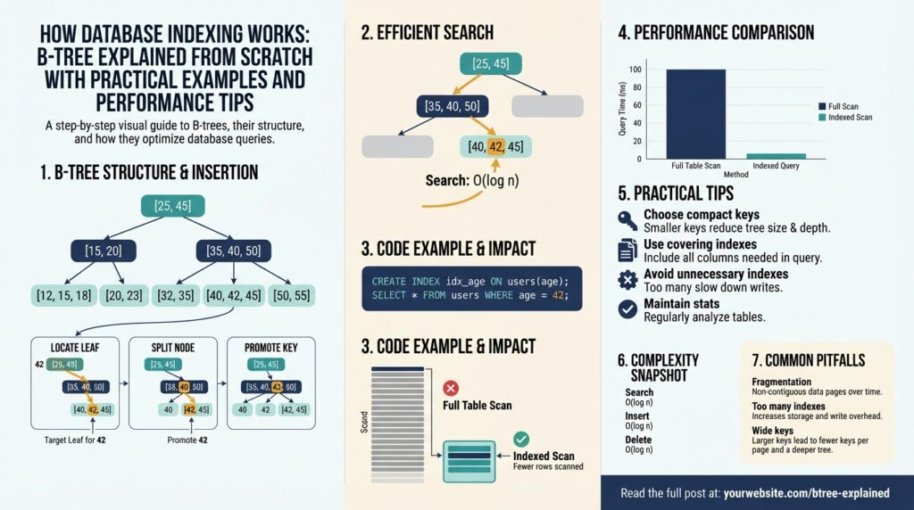
A node is a small, contiguous block that stores an ordered sequence of key values and either child pointers (internal nodes) or row references / record payloads (leaf nodes). In a B+Tree—what most databases implement—internal nodes store only keys plus pointers while all actual record references live in the leaves; leaves are linked together to support fast sequential scans. Fanout, which is the average number of children per internal node, depends on page size and entry size; higher fanout reduces depth and therefore the number of page reads for a lookup.
To see why fanout matters, do a quick calculation: available_bytes_per_page ÷ average_entry_size ≈ entries_per_node, and entries_per_node is an approximate fanout. For a typical 8KB page, subtract a small header and pointers; if each key+pointer costs ~16 bytes you might fit roughly 400–500 entries per node, giving a very shallow tree for millions of rows. That shallow depth is why point lookups hit only 2–4 pages in many real-world databases: one or two internal node pages and one leaf page.
Search and traversal are straightforward and predictable: we binary-search the keys inside a node to pick a child pointer, then descend until we reach a leaf and perform an in-node search or read the record. This produces O(log_f N) I/O complexity, where f is fanout; higher fanout reduces the logarithm’s base and thus the number of I/Os. Pseudocode looks like: search(node, key): i = binary_search(node.keys, key); if node.is_leaf return node.entry[i] else return search(node.child[i], key) — the constant work per node is what makes B-Tree seeks fast and deterministic.
Writes cause the interesting dynamics: inserts push keys into leaf nodes until a node overflows, at which point a page split occurs and a middle key is promoted to the parent. Page splits and merges are the tree’s rebalancing primitives; they keep height balanced but cause write amplification and can fragment locality. What causes frequent page splits? Small keys, heavy random inserts, and full pages without reserved space. Monitoring split rates often gives you an early signal that an index is degrading write throughput.
There are tuning knobs you can use to control those dynamics. Fillfactor (reserved free space per page) reduces immediate splits by leaving headroom for updates; prefix compression shrinks stored keys to boost fanout when keys are long; choosing a larger page size increases entries per node but may hurt cache efficiency. For high-insert workloads you typically set a lower fillfactor (e.g., 70–90%) to trade storage for fewer page splits; for mostly-read indexes you increase fillfactor to maximize density.
The internal layout explains common operational patterns you’ll see: shallow trees with linked leaves are excellent for range queries and ordered scans because leaves are physically contiguous and traversable without backtracking, and covering indexes can eliminate leaf-to-row lookups entirely. Conversely, hash indexes are faster only for exact matches and cannot serve range queries; when you ask “Why does a range query still read many pages?” check whether the index is clustered, whether keys are dense, and whether leaves have been fragmented by splits.
Understanding these fundamentals prepares us to interpret page-level statistics and to make specific tuning decisions. Next we’ll walk through page-split traces, show how to read per-index metrics, and demonstrate targeted adjustments—like rebuilding a heavily split index or changing fillfactor—to restore predictable performance.
Node structure and properties
B-Tree node layout determines the single biggest practical trade-off between lookup latency and write amplification, so we start here: a node is a fixed-size page that stores an ordered sequence of entries plus a small header and pointers, and those on-page choices define fanout and I/O per lookup. You should think in terms of bytes: page_size minus header bytes divided by average entry size gives an approximate entries_per_node, which is the effective branching factor that controls tree depth and read cost. How do node properties affect lookup latency and split frequency? Understanding the per-node accounting lets you answer that question quantitatively.
A node’s header and metadata are the first things we consider because they control consistency and traversal. The header typically contains node type (root/internal/leaf), level, free-space offset, and lsn/version data used by crash recovery and concurrency control; databases also store an item directory or slot array to manage variable-sized entries. Internal nodes hold only separator keys and child pointers so they maximize fanout, while leaf nodes store either row references or the actual payload in B+Tree implementations; that separation is why leaves are the bottleneck for payload locality and internal nodes are the bottleneck for tree depth.
Entry format and key encoding have outsized impact on fanout and fragmentation. Each entry cost equals key_bytes + pointer_bytes + per-entry overhead (alignment, tombstone flags, item headers), so prefix compression, fixed-width encodings, or compacting composite keys can materially increase entries_per_node. For example, with an 8KB page, a 128-byte page header, an average 24-byte key, and an 8-byte pointer, you get roughly (8192-128)/(24+8) ≈ 252 entries per internal node—clearly sensitive to average key length and alignment. We therefore prefer concise key encodings for high-cardinality indexes and reserve larger keys or covering payloads only when the query benefit justifies shallower trees.
Free space management and fillfactor are the operational knobs you use to control splits and page churn. Fillfactor—reserve percentage of each page kept free on creation—reduces immediate page splits for hot insert patterns by trading storage density for update headroom; conversely, a high fillfactor maximizes per-page fanout but increases split frequency under random writes. Additionally, fragmentation from deletes or MVCC dead tuples creates usable but noncontiguous free regions that can force page compaction or expensive rebuilds; monitoring per-page free-space distribution and split rates gives an early signal to adjust fillfactor or run targeted maintenance.
Page splits and merges are the mutation primitives you must reason about because they cause write amplification and change locality. When a leaf overflows we split it into two pages and promote a separator key to the parent, which can cascade; split semantics require updating sibling pointers (to keep leaf-linked lists contiguous) and writing a parent node change, so a single logical insert can force multiple page writes and WAL records. You can mitigate excessive splits by tuning fillfactor, batching inserts in key order (to preserve locality), or using bulk-load paths that build full pages upfront—techniques we use in ingestion pipelines to reduce operational noise.
Concurrency and durability interact with on-page structure in subtle ways that affect throughput. Databases use short-lived latches or latch-free algorithms to protect in-page structures during splits and pointer updates, while transactional locks and MVCC handle visibility at tuple level; that separation minimizes contention but means splits briefly serialize local writes. From a durability perspective, splits and node-level metadata changes create additional WAL volume because databases must log both new page contents and parent updates; design choices that increase fanout reduce WAL for lookups but can increase per-update log churn when splits occur.
Knowing these node-level properties informs practical tuning decisions and what to measure next. Calculate expected fanout from your real average key size, watch per-index split rates and free-space histograms, and set fillfactor to balance your insert pattern against read density; when keys are large, consider prefix compression or narrower surrogate keys to improve fanout. Building on this, the next step is to trace actual page splits and read per-page metrics so we can quantify the effect of these node properties on latency, I/O, and WAL volume.
Search, insert, delete operations
B-Tree search, insert, and delete behaviors determine most of the latency and write-amplification characteristics you’ll see in production, so start here: a B-Tree index gives you O(log_f N) seeks for point lookups and highly efficient sequential access for range queries because leaves are linked. When you issue a point lookup (for example, SELECT * FROM orders WHERE id = ?), the database binary-searches keys in a handful of internal nodes then reads the target leaf; that predictable descent is what makes index seeks consistently fast. How do you minimize page splits during heavy inserts? We’ll show concrete patterns and knobs you can use to control splits, WAL amplification, and the cost of deletes so you can tune indexes for your workload.
Search (lookup and range) behavior is straightforward but operationally important. For a point lookup we hit roughly tree_depth pages: one or two internal pages and the target leaf, so reducing average key size or increasing fanout directly reduces I/O per lookup. For range queries the engine traverses to the first leaf and then follows the leaf-linked list, producing mostly sequential reads — this is why B-Tree indexes shine for ORDER BY and BETWEEN filters. If you need index-only performance, design a covering index that contains all projected columns so the planner can avoid visiting table rows entirely.
Inserts are where theory meets cost: inserting into a leaf writes the leaf page and often updates parent metadata; if the leaf overflows a split occurs, promoting a separator key to the parent and possibly cascading. Ordered inserts (keys largely appended) keep writes localized to the rightmost leaf and avoid splits, while random inserts scatter writes across many pages and cause far more splits and I/O. Practical pattern: for high-throughput ingestion, bulk-load or insert in key order, lower fillfactor (e.g., 70–90%) to reserve space for updates, or use a staging table and a single bulk CREATE INDEX to build dense pages with minimal split churn.
A short pseudocode sketch clarifies insert dynamics:
insert(key): leaf = descend_to_leaf(root, key)
if leaf.can_fit(key): write_key_to_leaf(leaf, key)
else: split = split_leaf(leaf, key); promote_to_parent(split.separator)
That split_leaf step is the expensive part: it updates sibling pointers, writes two leaf pages, and logs parent updates. The result is additional WAL and temporary higher write amplification whenever splits are frequent.
Deletes interact with MVCC and garbage collection in many engines; logical deletion (tombstones or MVCC dead tuples) often leaves space that only a background vacuum/compaction reclaims. A delete typically marks a tuple as invisible and creates dead-row bookkeeping rather than immediately merging pages; only when free space piles up or neighboring pages become sparse will the tree perform merges. Therefore bulk delete patterns should be followed by VACUUM/REINDEX or table rewrite strategies on systems with MVCC, and consider setting fillfactor proactively if you anticipate heavy churn to reduce fragmentation.
Operational implications you should act on are clear: monitor per-index split rates, leaf write amplification, and WAL volume; if splits dominate, lower fillfactor, switch to bulk-loads, or change your key strategy (surrogate monotonic keys like sequences or time-based UUIDs can dramatically reduce random-split rate). Also weigh the read benefits of wide, covering indexes against the write costs—each additional indexed column increases per-write work and potential split pressure. When deletes accumulate, schedule compaction and maintain good statistics so the optimizer continues to choose index plans correctly.
Taking these ideas further, the next step is tracing splits and measuring I/O at page granularity so we can quantify how changes to fillfactor, key encoding, or insert ordering affect latency and WAL. With per-index metrics in hand you can iterate confidently: reduce random writes where possible, design covering indexes for hot read paths, and use maintenance windows to reclaim space after large deletions.
Practical SQL examples
Building on this foundation, we’ll translate B-Tree concepts into concrete SQL patterns you can try immediately to diagnose and fix slow queries. If you’ve ever asked “How do you make a query avoid a table scan?” the answer is usually a well-shaped index plus verification with EXPLAIN. Below are practical, production-minded SQL examples—composite indexes, partial and expression indexes, and covering variants—paired with guidance on when to use each so you can make data-driven indexing decisions without guessing.
Start with composite indexes that match your filter and ordering. When queries filter by one column and order by another, make the most selective and most-filtered column the leftmost key; ordering columns belong later in the key list to avoid an extra sort. For example, if you frequently run SELECT order_id, created_at FROM orders WHERE customer_id = ? AND status = ? ORDER BY created_at DESC, create an index that favors the frequent equality filters first:
CREATE INDEX idx_orders_customer_status_created ON orders (customer_id, status, created_at DESC);
This index serves the WHERE predicates and supplies the ordering so the planner can avoid a separate sort phase and potentially perform an index-only scan when the projected columns are present in the index.
When most traffic touches recent rows, use a partial index to reduce write amplification and storage. Partial indexes limit the indexed subset to rows that matter for the hot path, which both cuts maintenance cost and narrows the search space for queries. For example, if most analytic queries examine the last 30 days, build a partial index like this:
CREATE INDEX idx_orders_recent_status ON orders (status, created_at) WHERE created_at >= now() - interval '30 days';
This keeps the index small and cheap to update while still accelerating the majority of queries. Use partial indexes when predicates are stable and nearly always present in your queries.
Covering indexes eliminate lookups to the table by including non-key columns needed by the query; this enables index-only scans that read only index pages. When your query projects a few extra columns, use the INCLUDE (Postgres) or equivalent to create a covering index. For example, to serve SELECT created_at, total_amount FROM orders WHERE customer_id = ? entirely from the index, do:
CREATE INDEX idx_orders_cover_customer ON orders (customer_id, created_at) INCLUDE (total_amount);
We prefer covering indexes for hot read paths because they reduce random I/O; however, remember that every included column increases index size and write cost, so include only what the query actually needs.
Expression and functional indexes solve mismatches between how data is stored and how it’s queried. For case-insensitive lookups or normalized keys, index the function the planner will evaluate. A common pattern is lowercasing emails for authentication lookups:
CREATE INDEX idx_users_lower_email ON users (lower(email));
Then query with WHERE lower(email) = lower($1) to get an index-guided lookup. Expression indexes let you avoid redundant computed columns and keep the B-Tree compact by storing the indexed expression rather than duplicating application logic.
Always validate with EXPLAIN or EXPLAIN ANALYZE to ensure the planner uses the index as intended and to quantify gains. Run the original query, add the proposed index, then re-run EXPLAIN ANALYZE to compare actual logical reads, heap fetches, and elapsed time; look for “Index Only Scan” or a dropped “Seq Scan” as evidence of success. As we discussed earlier, monitor index bloat, split rates, and WAL volume after deploying indexes—if you see unexpected split churn, adjust fillfactor or consider bulk-loading strategies. Taking these SQL patterns into the profiler lets you iterate from hypothesis to measured performance improvement and prepares you to dig into page-level B-Tree internals next.
Performance tips and trade-offs
A sharp improvement in query latency often comes with a clear cost: every B-Tree index you add changes the read/write balance of your system. You gain fast, predictable seeks and efficient range scans, but you also increase write amplification, storage footprint, and maintenance complexity. Treat indexing as a capacity decision: weigh the query-frequency and selectivity benefits against the steady per-write overhead that every insert, update, or delete will now pay. If you want predictable performance under mixed workloads, explicit trade-off analysis is necessary before you create another index.
When should you add an index, and when should you avoid one? Add an index when a pattern is both frequent and selective enough to justify the per-write cost—common cases are hot lookup keys, join columns, and ordering keys that appear in ORDER BY or GROUP BY. Avoid indexing low-selectivity fields, or only index them as part of a composite key where combined selectivity is meaningful. We also have to consider operational constraints: if your pipeline sustains very high write throughput, favor partial indexes, limited includes, or delayed denormalized read tables over broad, heavy indexes that will throttle ingestion.
Page-split dynamics and node fill control are where theoretical costs become tangible. When lots of random inserts hit full leaf pages, page splits cascade and WAL volume spikes; to mitigate that, set a fillfactor that reserves headroom for updates (ALTER INDEX idx_name SET (fillfactor = 80);) or use bulk-loads that build dense pages in sorted order. Another lever is key design: monotonic surrogate keys (sequences or time-ordered IDs) concentrate writes and reduce split rate, while fully random primary keys scatter writes and amplify splitting. These choices directly affect write amplification, tree fanout, and steady-state latency, so measure split rates before and after any change.
Choosing index shapes forces explicit trade-offs among size, maintenance cost, and planner behavior. Covering indexes remove heap lookups and can yield index-only scans, but including additional columns increases index size and per-write work; partial indexes shrink maintenance scope but rely on stable predicates to be helpful. Composite indexes can replace multiple single-column indexes if you order columns by common filter patterns, but their leftmost-prefix semantics mean some queries won’t benefit. How do you decide? Prototype the most common queries, add minimal coverage, then expand to include columns only when the index demonstrably reduces heap fetches or avoids sorting.
You can’t manage these trade-offs without concrete measurements. Run EXPLAIN ANALYZE and compare logical reads, heap fetches, and elapsed time before and after index changes; look for “Index Only Scan” or a dropped “Seq Scan” as signs of success. Complement planner traces with index-level telemetry: index usage counters, WAL bytes attributable to index maintenance, and per-index split statistics (or equivalent engine metrics). If an index shows low use but high write cost, drop or convert it to a partial/index-on-expression; if an index improves a hot path, consider tuning its fillfactor, prefix compression, or switching to a clustered/index-organized table to improve locality.
Adopt an experimental rollout and measurement cycle rather than one-off changes. Create candidate indexes in staging, run representative workloads, and measure both query latency and write amplification; use feature flags or phased deployments to A/B test in production when safe. When a long-running delete or migration creates bloat, schedule maintenance windows for reindexing or table rewrites rather than letting fragmentation silently degrade performance. Taking this iterative, metrics-driven approach gives you repeatable evidence for each indexing trade-off and prepares you to apply deeper B-Tree internals tuning with confidence.