Why Feature Selection Matters in MLOps
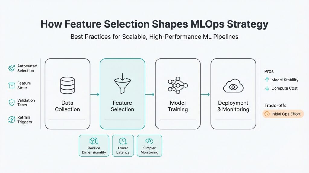
If your models are slow in production, expensive to run, or brittle to data drift, the root cause is often upstream: poor feature selection early in your pipeline. Feature selection is not an academic step you leave for model training; in MLOps it dictates latency, cost, and maintainability across ML pipelines from feature extraction to inference. When you prioritize the right features, you reduce input dimensionality, speed up training and scoring, and make monitoring and retraining practical at scale.
Building on this foundation, consider the operational costs that poorly chosen features impose. High-cardinality categorical fields, dense embeddings, or dozens of correlated telemetry signals multiply storage, network I/O, and inference compute. That translates directly into higher cloud bills, larger container images, and slower autoscaling behavior; during burst traffic you pay both in dollars and in SLA risk. We should evaluate features not only for signal but for compute footprint and serialization cost so models remain predictable under production load.
Beyond compute, feature selection shapes reproducibility and governance. If you rely on ad-hoc transformations scattered across training notebooks, you create feature drift between train and serve—the classic “it worked locally” failure mode. Centralizing selected features into a feature store or an agreed transformation library gives you lineage, versioning, and access controls so you can roll back, audit, or replay features during incident response. In regulated environments especially, pruning unnecessary or privacy-sensitive attributes early reduces compliance exposure and simplifies data retention policies.
How do you decide which features to keep when deploying pipelines at scale? Start with filter methods (correlation thresholds, mutual information) to remove noise, then use wrapper or embedded methods for interaction effects—L1 regularization for sparsity, tree-based importances for nonlinear signals, or SHAP values to capture global and local contributions. Complement metrics with operational tests: compute per-feature inference latency, network bytes for feature joins, and memory pressure for embeddings. For example, drop or quantize a timestamp-derived feature if it increases feature vector size but only marginally improves AUC; conversely, keep a compact signal that reduces model variance across cohorts.
Selection choices must integrate with monitoring and retraining. When you deploy a model, tag which feature selection method and hyperparameters produced that feature set so downstream pipelines can detect concept or feature drift and trigger retraining. We instrument per-feature distributions, missingness rates, and feature importance decay so automation can suggest re-including previously pruned signals or retiring ones that lost predictive power. Architecturally, separate online feature joins (low-latency scalar lookups) from heavy batch aggregates (complex joins computed offline) to avoid inflating your real-time stack.
Taking this concept further, treat feature selection as part of your MLOps contract rather than a one-off modeling step. That means codifying selection tests, operational cost budgets, and rollback rules into CI/CD for models: a candidate model fails the pipeline if its selected features push inference latency above threshold or increase cardinality beyond capacity. When we make selection decisions explicit and automated, we preserve model performance while keeping pipelines scalable, auditable, and cost-effective. In the next section we’ll translate these principles into concrete CI/CD checks and feature-store patterns you can implement immediately.
Assess Feature Importance and Cost
If your production costs creep up after a model rollout, the culprit is often a mismatch between predictive signal and operational expense — not just model architecture. We need to quantify both how much each feature contributes to predictive power and how much it costs to produce, serialize, and serve. Front-load this analysis in your MLOps workflow so feature importance and feature cost drive selection decisions early, not as an afterthought during optimization. How do you balance predictive power against operational cost?
Start by measuring predictive contribution with techniques that match your modeling context. Use model-agnostic permutation tests to get a baseline, SHAP (SHapley Additive exPlanations) or integrated gradients for local and global attribution when you need explainability, and model-specific importances (tree gain, coefficients) for a quick signal. Complement these with targeted ablation studies: retrain without a candidate feature and measure delta in validation metric and cohort variance. These approaches give you robust feature importance estimates and surface interaction effects that simple correlations miss.
Parallel to signal measurement, profile operational metrics at feature granularity rather than per-model aggregates. Run microbenchmarks to record per-feature inference latency, CPU/GPU FLOPs, memory residency, and network bytes for joins — measure cardinality and serialization overhead for categorical maps and embeddings. For example, a 512-dim embedding can dominate RAM and network cost compared with a handful of scalar telemetry counters; measure both the average and tail latencies because autoscaling and SLAs are driven by p95/p99 behavior. Treat missingness and preprocessing complexity (one-hot expansion, normalization pipelines) as part of feature cost, since they add runtime branches and IO.
Turn importance and cost into a usable score so you can compare apples to apples. A simple ratio works well in practice: score = ΔAUC / operational_cost, where operational_cost is a weighted sum of normalized latency, memory, and bytes transferred. For instance, if removing a feature reduces AUC by 0.004 but cuts per-request CPU by 20% and p99 latency by 8ms, the ratio favors keeping a high-impact low-cost signal. We regularly normalize metrics to account for scale (ms, MB, FLOPs) and include uncertainty bounds so we avoid overreacting to noise from small validation sets.
Make trade-offs explicit in training and CI: implement constrained optimization or cost-aware regularization to prefer compact representations. You can add a cost penalty to your loss, e.g., loss_total = loss_task + λ * cost(features) and tune λ via grid or multi-objective search. At deployment gating, encode hard rules: a PR that adds a feature must not increase p95 inference latency beyond the SLA or raise cardinality above configured limits. Automate a microbenchmark step in your model pipeline that returns a failing status and artifact if those thresholds are exceeded, so selection decisions are enforced by your MLOps pipeline rather than left to ad-hoc reviews.
Finally, treat this assessment as a living artifact: instrument feature-level telemetry in production, surface importance decay, and re-run ablation when concept drift or data-shift alerts trigger. We should tag models with the selection method and cost assumptions used at training time so downstream tooling can replay or roll back deterministically. By combining quantitative importance estimates, concrete operational measurements, and automated gates in CI/CD, you keep your pipelines performant and predictable while preserving the signals that matter most.
Prioritize Stable, High-Impact Features
Building on this foundation, we should default to features that are predictable in production rather than those that merely improve validation metrics. How do you pick signals that survive deployment, data shifts, and scaling? Start by distinguishing stability (features whose distributions and missingness remain consistent) from transient high-signal artifacts that overfit to a particular dataset. Prioritizing stability up-front reduces model churn, avoids costly rollbacks, and keeps your MLOps pipeline predictable under load.
Stable, high-impact signals combine sustained predictive value with low operational cost, and you should make both dimensions first-class in selection decisions. Stability means low importance decay over rolling windows, consistent cohort performance, and bounded missingness rates; high-impact means the feature yields measurable improvement in task metric after accounting for interaction effects. Treat feature importance and operational cost as paired metrics rather than competing trade-offs: a compact feature with small ΔAUC but near-zero latency or memory footprint can be more valuable than a large embedding that marginally lifts scores.
Quantify stability with automated checks that run during training and in production shadowing. Compute time-series metrics like Population Stability Index (PSI), Kolmogorov–Smirnov distance, and rolling SHAP importance to detect drift in distribution and contribution; a simple test is to compare a feature’s PSI across the last N windows and fail the build if PSI > threshold. Also measure operational cost per feature: p95 latency for lookup, bytes serialized for joins, and memory residency for embeddings. For example, a feature with stable SHAP ranking but a 512-dim embedding that increases p99 latency by 15ms should be re-evaluated or quantized.
Operationalize stability with gates, shadow launches, and feature contracts in your feature store. Enforce CI/CD checks that reject PRs where a candidate feature raises p95 inference latency beyond SLA, increases cardinality above configured limits, or exhibits PSI drift in a staging replay. Use feature flags and shadow traffic to validate a feature’s production behavior without routing live decisions; collect telemetry for missingness, lookup errors, and importance decay during the dark run so you can roll forward only when signals are stable and cost-effective. Tag models with the selection method and timestamped assumptions so rollbacks and deterministic replays are trivial.
When dealing with high-cardinality or dense vectors, apply pragmatic engineering patterns to preserve signal while lowering cost. Replace extremely wide one-hot encodings with hashing or learned embeddings and then compress them via PCA/SVD or distillation to fewer dimensions; consider product quantization for ANN searches or caching frequent-key lookups in memory to avoid remote joins. For categorical maps with millions of keys, evaluate a top-K fallback plus default bucket strategy and measure how often the fallback triggers—if it’s frequent, the raw cardinality is probably not adding value. These techniques let you keep meaningful representations without blowing up storage, network I/O, or autoscaling behavior.
Treat feature selection as a living contract between modeling and production teams rather than a one-off modeling step. We should continuously monitor feature importance decay, operational cost, and cohort-level performance, and wire those signals into automated retraining, canary rollouts, or feature retirement workflows. In the next section we’ll translate these stability criteria into concrete CI/CD checks and feature-store policies so your pipelines keep only the signals that matter while remaining scalable and auditable.
Automate Selection with Filters and Wrappers
Feature selection automation pays dividends in MLOps because manual pruning doesn’t scale when models, data sources, and SLAs change. Start by treating selection as a deterministic, auditable stage in your pipeline that produces a versioned feature set and measurable operational metadata (latency, memory, cardinality). When you do that, you can enforce reproducible experiments, run cost-aware comparisons, and gate deployments in CI/CD instead of relying on ad-hoc human judgment. This upfront discipline prevents the classic train/serve mismatch and keeps feature selection aligned with production constraints.
Filter methods are the cheap, high-throughput way to remove obvious noise before heavier analysis. Use fast statistics—correlation thresholds, variance filters, or mutual information—to drop features that add little signal or introduce multicollinearity, and calculate simple operational costs for each candidate (per-request bytes, lookup latency, embedding size). Because these computations are inexpensive, we run them on full datasets or rolling windows to catch transient correlations and to supply a compact candidate set to downstream, more expensive procedures. Integrating these metrics into an automated scoring sheet lets you compare predictive contribution against operational cost early in the pipeline.
Wrapper methods probe interactions and conditional importance by evaluating subsets against your actual learner; they’re slower but capture what filters miss. Techniques like recursive feature elimination (RFE), forward/backward selection, and sequential feature selection work well when paired with cross-validation or nested CV to avoid optimistic estimates. Run wrappers on the pre-filtered candidate pool and parallelize evaluations using joblib, Dask, or cloud batch workers to control wall-clock time; add early-stopping heuristics that abort searches when marginal utility falls below a configured Δmetric threshold. This two-stage approach—filters to shrink the search space, wrappers to refine the set—gives you the predictive gains of wrappers without their full computational cost.
Building on this foundation, codify the selection workflow into a pipeline that produces both a feature mask and an operational profile artifact. For example, implement a scikit-learn-style pipeline that applies SelectKBest (mutual_info) to reduce dimensionality, then runs an RFE loop with your production estimator; cache intermediate feature transforms and persist per-feature latency and bytes metrics alongside model artifacts. Sample pattern:
from sklearn.feature_selection import SelectKBest, mutual_info_classif, RFE
from sklearn.ensemble import RandomForestClassifier
from sklearn.pipeline import Pipeline

base = RandomForestClassifier(n_estimators=200)
filter_stage = SelectKBest(mutual_info_classif, k=100)
# run filter_stage.fit_transform(X, y) -> Xf, then run RFE on Xf with base
Persisting these artifacts lets downstream systems replay exact selection choices and measure production impact deterministically. Make the pipeline emit a JSON manifest that includes selected_feature_ids, selection_method, validation_delta, and operational_cost_score so that CI/CD gates can consume it automatically.
How do you ensure selection choices won’t break SLAs in production? Embed automated checks into your CI/CD: fail the build if the candidate feature set increases p95 inference latency beyond SLA, raises cardinality above a configured limit, or causes memory footprint regression above a threshold. Use shadow traffic and canary deployments to validate selected features under real load without affecting live decisions, and collect feature-level telemetry (missingness, PSI, importance decay) during the dark run. If telemetry shows unacceptable drift or cost spikes, trigger automated rollback or a retraining job that re-runs the filter+wrapper pipeline with updated data.
In practice, a common pattern is to prefer cost-aware wrappers: augment the evaluator’s objective with a penalty term so selection optimizes predictive power and operational cost simultaneously. For example, tune a hyperparameter λ in loss_total = loss_task + λ * cost(features) during wrapper search to derive compact, high-impact sets tailored to production budgets. When you combine this with versioned manifests and feature-store contracts, you create an automated, auditable path from selection experiments to production rollout. That automation preserves model quality while enforcing MLOps guardrails and sets up the next stage: CI/CD checks and feature-store policies that ensure the chosen features remain safe and scalable in production.
Feature Stores, Versioning, and Lineage
Feature store is where your feature selection choices stop being ephemeral notes in a notebook and start being enforceable contracts for production. If you’ve ever faced a “worked-in-dev, failed-in-prod” incident, it’s usually because the feature schema, transformation code, or freshness assumptions changed without a trace. How do you ensure feature changes don’t silently break production models? Treat the feature store as the single source of truth for feature definitions, operational metadata, and access controls so every consumer—training job, scoring service, or auditor—reads the same contract.
Versioning feature definitions is the practical foundation for reproducibility and safe rollouts. Every feature should carry a semantic version plus an immutable identifier (for example, feature_id:v2026-02-18 or a git commit SHA) and a timestamped manifest that records the transform code, dependencies, and expected cardinality. Use versioning to gate deployments: a model artifact must declare the exact feature versions it expects, and CI should fail if a candidate feature set upgrades a dependency without passing production microbenchmarks. This makes drift visible and enables deterministic replays for debugging or regulated audits.
Make manifests machine-readable and include operational metadata so automation can consume them downstream. A minimal manifest might be a small JSON object with fields like selected_feature_ids, feature_versions, materialization_strategy, and operational_cost_estimate. For example:
{
  "model_id":"fraud-scorer:v2",
  "features":[{"id":"tx_amt_avg","ver":"v1.3"},{"id":"user_age_bucket","ver":"v2.0"}],
  "materialization":"online_cache",
  "p95_latency_ms":4.2
}
Persisting that manifest with the model artifact and the feature-store registry makes rollbacks and audits deterministic and automatable.
Lineage is the breadcrumb trail that links raw inputs to engineered features, to model inputs, and finally to predictions. Record lineage at two levels: transformation lineage (what SQL or code produced this column) and provenance lineage (which raw dataset version, ingest job, or external lookup produced the inputs). When an alert fires—e.g., sudden importance decay or cohort failure—you should be able to trace backward from a model prediction to the exact raw files, transformation commit, and feature version used in scoring. That traceability is the backbone of incident response and model forensics.
Operationally, implement lineage and provenance using immutable artifacts and event logs. Emit a lineage record whenever a feature is materialized or updated: include feature_id, version, transform_commit, source_dataset_version, and job_run_id. Store these records in a tamper-evident event store or a feature registry table that CI/CD and monitoring systems can query. Couple this with tight versioning: the same transform_commit that’s recorded in lineage should exist in your Git history, packaged in the model image, and referenced in the manifest so everything links end-to-end.
Consistency between online and offline views is critical for low-latency inference and accurate retraining. Materialize features deterministically with atomic updates—apply shadow writes, promote atomically on successful backfill, and maintain TTLs so freshness guarantees are explicit. Dual-write patterns (writing both to the feature store and the online cache) must be reconciled by a materialization daemon that verifies counts and cardinality before promoting a new feature version. These engineering controls avoid train/serve skew and keep production latency predictable.
Tie lineage and versioning to monitoring and automated rollback logic so you can act when features decay or cost budgets are breached. Surface feature-level telemetry (PSI, missingness, lookup errors, and p99 latency) and map those metrics to the manifest and lineage records; when thresholds trip, trigger canary rollbacks or retraining runs that consume the exact historical feature versions. This lets you answer operational questions quickly—what changed, when, and which model runs used the altered feature—without manual forensics.
Building on this foundation, make the feature store, versioning, and lineage artifacts first-class inputs to your CI/CD gates and retraining workflows. When your pipeline rejects a PR because the feature manifest increases p95 latency above an SLA or because lineage shows an unsupported external dependency, you prevent costly failures downstream. In the next section we’ll translate these constraints into concrete CI checks and feature-store policies that automate enforcement and keep models reproducible, auditable, and scalable.
Monitor Drift, Retrain, and Governance
Building on this foundation, treat monitoring for drift, retraining, and governance as the operational backbone that enforces your feature selection choices in production. Feature selection and MLOps constraints should be visible at runtime: per-feature telemetry, operational cost metrics, and model-level performance live together in your observability layer. Instrumentation that captures PSI, p95 latency, lookup-errors, missingness, and SHAP-based importance decay lets you correlate predictive degradation with the exact features and transforms that caused it. When you make these signals first-class, automated responses—rather than manual firefighting—become feasible.
Start by defining the signal set you will monitor per feature and why each metric matters. For distributions, compute Population Stability Index (PSI) and KS distance on rolling windows to detect covariate drift; for contribution, track rolling SHAP medians and importance rank shifts to detect importance decay; for ops, measure p95 lookup latency, cardinality, and bytes transferred so cost regressions surface. Capture missingness and lookup-error rates because production joins and late-arriving keys often cause subtle train/serve skew. Persist these metrics with the same timestamps and feature-version metadata you use in your feature store so alerts map directly to manifests and lineage.
How do you decide when to retrain or intervene? Define multi-axis triggers that combine predictive, feature, and operational thresholds: for example, trigger an investigation if model AUC drops by X, or if a feature’s PSI exceeds Y for N windows, or if a top-k feature loses more than Z% SHAP contribution while its lookup latency increases. Use adaptive baselines that discount seasonal shifts and require sustained deviation to avoid noisy churn. Pair statistical alerts with cost-aware guards—if a feature’s importance increases but its operational cost would breach SLA, open a gated PR that requires either compression, quantization, or a fallback strategy before rollout.
Automate retraining as a staged workflow that respects your feature-store contracts and CI/CD gates. Implement event-driven retrain pipelines for concept-shift scenarios and scheduled retrains for label-latency domains; include a data-sampling strategy that preserves temporal coherence and minority cohorts. When retraining, pin feature versions from the manifest, re-run the filter+wrapper selection with the same cost-aware penalty, and produce a new selection manifest that CI can microbenchmark. Release the candidate via shadow traffic and a canary rollout, collect feature-level telemetry during the dark run, and only promote once both predictive and operational SLAs are satisfied.
Governance ties this loop together so you can audit, roll back, and justify decisions to stakeholders and regulators. Enforce feature contracts in the feature store: immutable feature IDs, semantic versions, materialization strategy, and an operational-cost estimate stored in the manifest. Restrict write and approve permissions on production feature definitions, require transformation commits to be linked to lineage records, and make manifests machine-readable so CI/CD gates can reject PRs that would violate latency, cardinality, or compliance budgets. Maintain tamper-evident event logs for materialization runs so forensic traces link predictions back to the exact raw files, transform commit, and feature version.
Consider a concrete scenario: a fraud model where a geolocation-derived feature suddenly drifts after a partner changes their API format. Your alerting flags a PSI spike and a SHAP importance drop while p99 lookup errors climb. The pipeline automatically blocks new feature-version promotions, triggers a retrain job that excludes the unstable geolocation input, and creates a compact fallback representation (top-K buckets plus default). After shadow validation and a successful canary, the new model and an updated manifest are promoted, and the lineage records the rollback window and decision rationale for auditors.
Taking these practices together, we turn feature selection from a one-time modeling choice into a governed, observable lifecycle that keeps models reliable and cost-effective. By automating drift detection, conditioning retraining on both signal and operational budgets, and enforcing manifests and lineage through CI/CD, you reduce incident time-to-recovery and maintain auditable controls. In the next section we’ll translate these governance rules into concrete CI/CD checks and feature-store policies you can implement immediately.