Why Hyper-Connections Fail
Building on this foundation, the core reason Manifold-Constrained Hyper-Connections break in practice is a misalignment between theoretical geometry and the empirical representations your model actually learns. When you design hyper-connections that assume neat, low-dimensional manifolds, you implicitly require that upstream and downstream latent spaces share compatible topology and scale. If those latent spaces instead carry anisotropic curvature, multi-modal clusters, or differing intrinsic dimensions, the hyper-connection becomes a brittle bridge rather than a robust mapper. This mismatch surfaces early in training as noisy activations and later as persistent performance gaps across tasks.
A dominant failure mode is manifold mismatch: the mapping you impose through a hyper-connection is not expressive in the right ways. You can parameterize an mHC with a linear projection, an MLP, or a constrained orthogonal map, but each choice encodes assumptions about curvature and local isometry. When the true latent geometry requires nonlinear transport or density-preserving transforms, a misspecified hyper-connection distorts representations, causing downstream layers to learn compensatory weights. Consequently, you see representational collapse, where different inputs map to indistinguishable downstream states, or fragmentation, where semantically close examples land in separate regions of the target manifold.
Optimization and training dynamics create another set of predictable failures. The loss landscape induced by a hyper-connection often introduces saddle points and narrow valleys that decouple gradients between modules; this makes joint training unstable and sensitive to learning rate schedules. Vanishing or exploding gradient flow across the mHC is common when norms and activation statistics differ between connected modules, and the usual fixes—gradient clipping or naïve normalization—can mask rather than resolve the underlying geometry problem. As a result, parameter updates oscillate or collapse to degenerate minima, and your validation metrics stop improving even though per-module losses decrease.
Architectural and data issues amplify these problems in real systems. If you connect a high-capacity convolutional encoder to a lightweight transformer head with a single dense hyper-connection, the capacity mismatch forces one side to overfit while the other underfits. Domain shift between training and deployment data further exposes fragile hyper-connections: a small change in input distribution can move latent points off the assumed manifold and break alignment. Regularization choices—dropout, batch normalization, weight decay—interact nonlinearly with manifold constraints, so a recipe that works for isolated modules may destabilize the full mHC architecture when combined.
Practical engineering details are surprisingly decisive. Numerical precision, initialization, and the order of operations in residual paths all affect whether a hyper-connection converges to a meaningful map. If you initialize the projection to small weights, you may inadvertently encourage identity collapse; if you initialize too large, you’ll produce spurious high-curvature mappings that cause training instabilities. Monitoring per-layer activation spectra, singular value distributions of projection matrices, and alignment statistics (e.g., cosine similarity between paired latent pairs) gives early warning signs that the manifold assumption is failing before validation loss degrades.
How do you detect when a hyper-connection has failed during training? One practical approach is to run contrastive or probe-based alignment checks: sample paired inputs that should be nearby on the target manifold and measure distance preservation across the mHC. In a multi-modal example—say, connecting image latents from a ResNet to text latents in a transformer—if neighbor structure is not preserved after the hyper-connection, you know the mapping is misaligned. To mitigate this, we often add a small alignment module (orthogonalizing layers or learned transport maps), use contrastive pretraining to align marginals, or introduce local Jacobian regularizers that encourage isometry in critical regions of the manifold.
Recognizing these failure modes changes how you design and validate Manifold-Constrained Hyper-Connections in real projects. Rather than treating an mHC as an innocuous wiring choice, instrument it, measure geometry-preservation metrics, and stage training (pre-align, then fine-tune jointly) to reduce brittleness. In the next section we’ll examine concrete alignment layers and training schedules that restore reliable gradient flow and preserve manifold structure across modules.
Core Idea of mHC
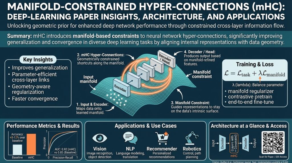
Building on this foundation, the core idea behind Manifold-Constrained Hyper-Connections is simple in statement and subtle in execution: treat the connection between module latents as a learned geometric transport that must respect the local shape and density of the source and target manifolds. We think of the hyper-connection not as a generic shortcut or a feature projection, but as a constrained map whose role is to preserve neighborhood structure, important curvatures, and task-relevant metrics so downstream modules can operate on consistent representations. When that map enforces the right geometric priors, you avoid the brittle mapping and compensatory learning described earlier.
At a technical level, an mHC explicitly encodes constraints on the Jacobian, topology, or volume change of the mapping so that local distances and relative orientations are preserved where it matters. Local isometry constraints (preserving small distances) guard against neighbor-structure collapse, volume-preserving constraints prevent density distortion that breaks probabilistic heads, and topology-aware constraints ensure multimodal clusters remain separable after transport. Framing the hyper-connection as a transport operator clarifies why optimization and initialization interact with geometry: you’re not just learning weights, you’re learning a differential map whose singular values and Jacobian spectrum determine stability across training.
You can implement that transport with several practical primitives depending on how wild the latent geometry is. If source and target manifolds are near-isometric, an orthogonal linear map or an orthonormal projection often suffices and is cheap to train. When curvature or density mismatch is moderate, a small constrained MLP with an explicit Jacobian regularizer gives the flexibility you need without overfitting. For severe topology or density differences, use invertible architectures or normalizing flows (coupling layers, RealNVP / NICE patterns) or approximate optimal-transport layers (Sinkhorn maps) that explicitly model volume change. Attention-based cross-modal transport can be effective when correspondences are sparse and context-dependent rather than globally geometric.
Training strategy and regularization enforce the manifold constraints in practice. Pre-align the marginals with a contrastive or maximum mean discrepancy (MMD) objective to give the hyper-connection a good initialization, then fine-tune jointly with a geometric regularizer such as ||J^T J – I||_F (which penalizes deviation from local orthonormality). How do you choose the right constraint for your scenario? If neighbor preservation matters most, prioritize local isometry losses; if probabilistic heads require calibrated densities, favor flow-like, volume-aware mappings. Monitor singular-value spread, cosine alignment of paired latents, and local reconstruction error to detect mismatch early.
To make this concrete, imagine connecting a 512-d ResNet image latent to a 768-d transformer text latent. A pragmatic recipe is: initialize an orthogonal projection to expand 512→768, add a shallow coupling-flow (2–4 coupling layers) to model density differences, pretrain with a contrastive alignment loss on paired image-text examples, and then fine-tune the entire stack with a small Jacobian penalty and spectral norm clipping. A compact PyTorch pattern for the Jacobian regularizer looks like this:
# x: (batch, d) -> y: (batch, d') via mapping f
y = f(x)
# compute jacobian-vector products efficiently
grads = torch.autograd.grad(y, x, grad_outputs=torch.ones_like(y), create_graph=True)[0]
JtJ = (grads.transpose(0,1) @ grads) / x.size(0)
iso_loss = ((JtJ - torch.eye(JtJ.size(0), device=JtJ.device))**2).sum()
loss = task_loss + lambda_iso * iso_loss
We recommend instrumenting these mappings: track singular-value distributions of the linear parts, alignment recall on paired samples, and local distortion metrics during pretraining and fine-tuning. Taking this geometric view of Manifold-Constrained Hyper-Connections changes design from picking a convenient projection to selecting a transport hypothesis, which we then validate empirically and refine with targeted regularizers and staged optimization before integrating into larger systems.
Mathematical Formulation
Building on this foundation, we now write the mHC mapping as an explicit, constrained operator so you can reason about stability, volume change, and topology in a single mathematical framework. Let M_s ⊂ R^m and M_t ⊂ R^n be the source and target data manifolds with intrinsic dimensions k_s and k_t; parameterize the hyper-connection as f_θ: R^m → R^n (learned transport) that we want to restrict on M_s to map into M_t while preserving task-relevant geometry. The primary object that controls local behavior is the Jacobian J_f(x) = ∂f_θ(x)/∂x: tangent vectors in T_xM_s are transported by J_f(x) into tangent directions in T_{f(x)}M_t, so constraints on J_f are the natural instrument for enforcing local isometry, volume control, and invertibility. Manifold-Constrained Hyper-Connections therefore become constrained-optimization problems over f_θ with Jacobian-aware penalties and structural choices that match the expected geometry of the two manifolds.
To preserve neighborhood structure where it matters, impose a local isometry condition on tangent spaces: for x drawn near M_s we want J_f(x)^T J_f(x) ≈ I_k (or, more generally, ≈ P_{T_x}, the projector onto the intrinsic tangent basis). In practice we penalize deviation with a Frobenius-norm term such as L_iso = E_x ||J_f(x)^T J_f(x) – I_k||_F^2; when the singular values σ_i(J_f(x)) cluster around 1, small distances and relative orientations are preserved and downstream modules see consistent local geometry. Expressing the constraint in singular-value terms also gives clear diagnostics: a wide spread in {σ_i} signals stretch/compression and predicts gradient flow issues or representational collapse, while σ_i ≈ 1 indicates near-isometry.
Volume and density preservation matter when probabilistic heads expect calibrated likelihoods or when the downstream loss is sensitive to mass transport. A natural volume penalty is L_vol = E_x (log|det J_f(x)| – c(x))^2, where c(x) is a target log-volume change (zero for volume-preserving maps). When you can afford invertible blocks, use architectures with tractable log-determinant terms (normalizing flows) so the volume penalty is exact and gradients are stable; density-aware flows like RealNVP give you an explicit log|det J| term you can optimize directly. Enforcing or penalizing log|det J| reduces density distortion that otherwise breaks probabilistic calibration in downstream modules. (research.google)
Topology-aware constraints require thinking beyond local linearization: if clusters in M_s must remain separable after transport, f_θ should be (locally) bijective on relevant neighborhoods or implemented with invertible components so it cannot fold distinct clusters into the same image. When topology mismatch is severe, incorporate invertible architectures or optimal-transport regularizers—entropic optimal-transport (computed efficiently with Sinkhorn iterations) provides a soft, global alignment objective that complements local Jacobian penalties by matching marginals and preserving cluster structure across distributions. Combining a Sinkhorn alignment term with local J-penalties gives a practical hybrid: local isometry enforces neighbor preservation while Sinkhorn ensures that global mass moves coherently. (papers.nips.cc)
How do we enforce these constraints efficiently during training? Compute Jacobian-vector products using automatic differentiation and approximate trace-like quantities with stochastic probes: E_v ||J_f(x)v||^2 equals tr(J_f(x)^T J_f(x)) when v is Gaussian, so Hutchinson-style estimators let you approximate Frobenius and trace terms with O(1) backward passes per probe instead of forming full Jacobians. Recent variance-reduced trace estimators (Hutch++ family) further reduce probe counts when trace accuracy matters, making Jacobian-aware regularizers practical at scale for typical batch sizes. These stochastic estimators let you implement L_iso proxies such as E_{x,v} (||Jv||^2 – ||v||^2)^2 that converge to the desired isometry penalty without materializing J. (pubmed.ncbi.nlm.nih.gov)
Putting everything together, the mHC learning objective becomes a weighted sum: L(θ) = L_task + λ_iso L_iso + λ_vol L_vol + λ_ot L_sinkhorn + λ_reg R(θ), where each weight reflects how much local distance, volume, and global transport matter for your downstream head. Choose structural primitives (orthogonal linear layers, constrained MLPs, coupling flows) to make those penalties meaningful: orthogonality biases J toward isometry, small constrained MLPs control curvature, and flows expose exact log-determinants for volume control. These mathematical primitives give you explicit levers—singular-value targets, trace estimators, log-det penalties, and Sinkhorn costs—to diagnose and correct manifold mismatch before brittle behavior emerges, and they naturally lead into practical alignment layers and staged training schedules described next. (deeplearningbook.org)
Sinkhorn Projection and Constraints
Building on this foundation, entropic optimal transport via Sinkhorn gives you a practical, differentiable way to align marginals between source and target latents while preserving cluster mass. The Sinkhorn algorithm computes a soft transport plan between batched latent distributions using entropic regularization, so it fits naturally as a global alignment term alongside local Jacobian penalties and volume constraints. Using a Sinkhorn projection early in pretraining can reduce large-scale mass mismatch that local isometry losses cannot correct, and entropic smoothing controls gradient variance during stochastic optimization. How do you decide when to lean on this global alignment versus local constraints?
Start by thinking of the transport objective in batch form: you construct a cost matrix C between a batch of source embeddings X and a batch of target embeddings Y, then run Sinkhorn iterations to obtain a row- and column-normalized transport matrix P. Entropic regularization (often denoted ε) makes the optimization strictly convex and yields P via iterative matrix scaling, which you can implement with log-domain stabilizers to avoid underflow. The resulting plan P is differentiable with respect to X and Y, so adding a Sinkhorn loss term L_ot = ⟨P, C⟩ to your training objective gives a direct signal that moves mass in a globally coherent way without enforcing local bijectivity.
In practice, you’ll combine this global plan with local Jacobian-aware constraints rather than replacing them. Use a weighted objective L = L_task + λ_iso L_iso + λ_vol L_vol + λ_ot L_ot and tune λ_ot so the transport term corrects gross marginal mismatch without overwhelming gradient signals that preserve tangent structure. Low ε (weak entropic smoothing) makes the plan near-deterministic and can inject high-variance gradients that destabilize training; higher ε smooths the plan and improves optimization but sacrifices sharp cluster separation. A practical heuristic is to start with larger ε during pre-alignment, then anneal it down while reducing λ_ot as the Jacobian penalties take over, giving you a staged schedule that respects both global correspondence and local isometry.
Implementing a Sinkhorn-based projection for a hyper-connection is straightforward and computationally efficient at batch scale if you follow a few engineering rules. Compute the cost C_{ij} = d(X_i, Y_j)^2 or a cosine-based surrogate if your latents are normalized; apply log-sum-exp stabilized Sinkhorn iterations for T steps (typical T ∈ [20,100] depending on ε) to get P; then form a barycentric mapped point X̂i = ∑_j P Y_j to use as the transported representation. This barycentric mapping acts as a soft projection of source points into the convex hull of the target batch and integrates cleanly into backprop because autograd flows through both the Sinkhorn iterations and the barycentric sum. Use mixed precision carefully and clamp exponentials in the log-domain to keep GPU numerics stable.
Expect trade-offs in compute and statistical fidelity. Mini-batch Sinkhorn approximates full-distribution OT but introduces sampling bias: the transport plan reflects batch composition, so anchor selection or persistent memory banks can stabilize alignment across iterations. Monitor the entropy of P and the effective support size: a rapidly collapsing entropy indicates the plan is becoming nearly deterministic and may magnify gradient spikes, while persistently high entropy suggests under-alignment. Combine these diagnostics with singular-value spectra of the linear parts of the hyper-connection to see whether global transport is correcting topology mismatch or merely masking local distortion.
When should you use this approach? Choose a Sinkhorn-enabled alignment when source and target manifolds exhibit cluster-level drift, multi-modal mass shifts, or when downstream probabilistic heads require coherent marginals; prefer local Jacobian constraints when neighborhood preservation and tangent fidelity are paramount. We can tune the entropic regularization, plan iteration count, and λ_ot as levers to trade optimization stability against alignment sharpness. Taking this blended approach—global Sinkhorn plans plus local isometry and volume penalties—gives you a robust, diagnosable pathway to restore manifold alignment before we move on to concrete alignment layers and staged training schedules.
Efficient Implementation Strategies
Building on this foundation, the hardest engineering step is turning geometric prescriptions for Manifold-Constrained Hyper-Connections into implementations that scale and train reliably. You need answers to practical questions: how do you enforce Jacobian-aware penalties without blowing memory, how do you combine global Sinkhorn alignment with local isometry losses, and how do you stage optimization so gradients remain informative? This section gives concrete patterns and runnable ideas you can drop into a PyTorch-style pipeline to make mHCs (and any hyper-connection) robust in real projects.
Start by selecting a structural primitive that matches the expected manifold mismatch; this choice sets the implementation budget. If source and target are near-isometric, prefer an orthogonal linear expansion (cheap matrix multiply, stable singular values) and initialize with an SVD-based orthonormalizer to avoid identity collapse. When moderate curvature or density differences exist, use a shallow constrained MLP with spectral normalization or parameterized orthogonality (e.g., Cayley/Householder layers) to limit pathological singular-value spread while keeping compute low. For severe density/topology differences, invest in small coupling-flow blocks (2–4 layers) so you can compute exact log-determinants during fine-tuning and avoid ad hoc volume approximations.
Pipeline and optimizer choices matter as much as architecture. Stage training: pre-align marginals (contrastive loss or mini-batch Sinkhorn) with the hyper-connection weights frozen or lightly updated, then unfreeze and fine-tune with Jacobian and volume penalties added. Use an adaptive optimizer with decoupled weight decay (AdamW) and a lower learning-rate multiplier for the hyper-connection than for heads to prevent fast overfitting. Apply gradient clipping and spectral-norm clipping on linear parts to keep singular values within a controlled band; this reduces oscillation in the loss landscape and stabilizes gradient flow across modules.
You can compute Jacobian-aware regularizers efficiently with stochastic probes rather than forming full Jacobians. Hutchinson estimators let you approximate tr(J^T J) with a single Jv product per probe; use Gaussian or Rademacher probes and average across a few draws per mini-batch. A compact PyTorch pattern looks like this:
# x: (B, d) -> y = f(x)
v = torch.randn_like(x)
Jv = torch.autograd.grad(y, x, grad_outputs=v, retain_graph=True, create_graph=True)[0]
trace_est = (Jv.square().sum(dim=-1) / v.square().sum(dim=-1)).mean()
iso_loss = (trace_est - 1.0).pow(2)
Use Hutch++ if trace variance becomes a bottleneck; in practice 1–4 probes per batch often suffices. Combine these probes with mixed precision and gradient checkpointing to keep memory use acceptable on large batches.
Make Sinkhorn alignment practical at batch scale by stabilizing both statistics and compute. Use cosine-normalized latents and a squared-cost surrogate when euclidean distances are noisy; clamp log-domain exponentials and run T∈[20,80] iterations with entropy annealing (start high ε, reduce toward target). To reduce sampling bias, maintain a small persistent memory bank or momentum queue of target embeddings so each batch sees a broader empirical marginal; compute barycentric projections from the stabilized plan and feed them to the downstream head during pre-alignment. Monitor plan entropy and effective support size; if entropy collapses quickly, increase ε or introduce stochastic anchors to avoid spiky gradients.
Instrumentation is non-negotiable: monitor singular-value histograms of linear blocks, per-batch alignment recall on paired examples, the distribution of log|det J| when available, and Sinkhorn entropy. Automate lambda schedules: decrease λ_ot as Sinkhorn pre-alignment completes, then anneal λ_iso more slowly while you fine-tune task loss. Surface these metrics in lightweight summaries (per-step scalars and moving-window percentiles) so you can detect representational collapse before validation metrics degrade.
Finally, design the hyper-connection as a pluggable module with two runtimes: a full training forward that computes transport, probes, and regularizers, and an optimized inference forward that fuses orthogonal linear layers, drops probes, and replaces coupling flows with cached barycentric mappings or distilled linear approximations when acceptable. This keeps training expressive while making deployment efficient and predictable. Taking these implementation strategies together lets you operationalize mHCs: we preserve the geometric guarantees you designed for, while keeping compute, memory, and optimization stable enough for production workflows.
Benchmarks and Practical Applications
Manifold-Constrained Hyper-Connections (mHC) change the evaluation game because they require geometric, not just predictive, fidelity. If you treat a hyper-connection as a black-box projector, you miss failure modes that show up only in geometry-aware diagnostics; therefore our benchmarks must exercise both task performance and manifold-preservation properties. Building on the earlier discussion about Jacobian penalties and Sinkhorn alignment, we recommend benchmark suites that stress topology, local isometry, and downstream utility rather than reporting a single scalar accuracy. This reframing lets you compare transport hypotheses (orthogonal expansions, constrained MLPs, coupling flows) on equal footing across realistic workloads.
Design the experimental protocol so it isolates the hyper-connection’s role in a staged training pipeline. Start with pre-alignment experiments where you freeze encoders and measure how quickly a newly initialized hyper-connection achieves alignment under contrastive or Sinkhorn objectives; next, unfreeze and fine-tune jointly while enabling Jacobian and volume penalties to observe stability. Include ablations that remove one regularizer at a time (λ_iso, λ_vol, λ_ot) and variants that replace constrained primitives with unconstrained baselines; these controlled comparisons reveal which geometric lever is responsible for gains and which simply masks mismatch. We also recommend measuring optimization sensitivity by sweeping learning-rate multipliers for the mHC and varying probe counts for Hutchinson estimators to quantify probe variance versus regularization strength for the trained map.
How do you measure mHC effectiveness in a way that’s meaningful for production systems? Use a mix of geometric and application metrics: alignment recall@k on paired validation sets to capture global correspondence; average local distortion (mean ||f(x+δ)−f(x)||/||δ|| over tangent-like perturbations) to capture local isometry; singular-value dispersion of linear blocks to detect stretch/compression; and distributional log|det J| statistics when using flow-like components to assess volume fidelity. Complement these with downstream metrics—task loss, negative log-likelihood for probabilistic heads, calibration error, fine-tuning steps-to-convergence, and practical measures like additional FLOPs and end-to-end latency introduced by the hyper-connection. Tracking both geometry and utility uncovers trade-offs you can tune rather than obscure.
Apply the suite to representative scenarios so results translate to real projects. For cross-modal retrieval (image↔text), benchmark alignment recall and retrieval latency while varying entropic regularization ε in your Sinkhorn stage; observe whether stronger ε speeds optimization at the cost of cluster separation. For modular transfer—plugging a high-capacity vision encoder into a lightweight task head—measure how much the mHC reduces head fine-tuning steps and whether it prevents representational collapse by preserving neighbor structure. For continual learning or domain-shift tests, track how quickly the mHC re-aligns with a small replay buffer and whether Jacobian penalties mitigate catastrophic folding when new modes appear. These scenarios mirror common engineering problems and show where Manifold-Constrained Hyper-Connections provide the biggest leverage.
Practical application requires understanding operational trade-offs and deployment patterns. When inference latency is critical, we recommend training with expressive flows or Sinkhorn plans but distilling the transport into a fused orthogonal linear layer or a cached barycentric mapping for the fast path; this preserves most geometric gains while reducing runtime cost. When probabilistic calibration matters—density-preserving heads or likelihood-based ranking—favor invertible primitives with tractable log-determinants even if they add training overhead, because volume fidelity directly affects downstream calibration. Instrumentation remains essential: expose singular-value histograms, plan entropy, and distortion percentiles in CI so regressions in geometric fidelity surface before they become service-impacting.
Taking benchmarks beyond accuracy gives you actionable signals: which constraint to strengthen, where to trade compute for fidelity, and when to distill for production. As we move into alignment layers and staged schedules, we’ll use these exact metrics to pick λ schedules, probe counts, and the point at which global Sinkhorn alignment hands off to local Jacobian control—so you can reproduce stable, geometry-aware hyper-connections in your systems.