Introduction to SQL Window Functions
When you need to calculate running totals, rank users, or deduplicate rows without writing complex self-joins, SQL window functions unlock a concise, performant solution. SQL window functions like ROW_NUMBER, RANK, and DENSE_RANK let you compute values across a set of rows related to the current row while preserving row-level context — we can rank, aggregate, or compute moving sums without collapsing results into a single group. This section introduces the core idea and practical patterns so you can start using these ranking functions immediately in production queries.
Building on this foundation, think of a “window” as a movable frame that defines which rows are visible to a calculation for each output row. Partitioning splits the result set into groups (PARTITION BY) and ordering defines the sequence inside each group (ORDER BY); the OVER(…) clause binds these definitions to the function. These concepts let you express questions like “what is the rank of this sale within its region this quarter?” in a single SELECT, and they avoid costly GROUP BY reshaping when you still need row-level detail.
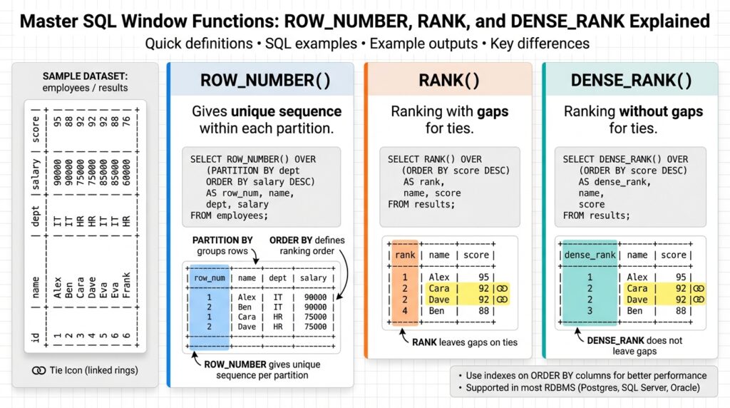
ROW_NUMBER, RANK, and DENSE_RANK solve similar problems but differ in tie handling and result semantics. ROW_NUMBER assigns a unique sequential integer per partition with no ties — useful when you need deterministic row selection. RANK leaves gaps when ties occur (for example, two rows tie for rank 1, the next gets rank 3), which preserves ordinal positions. DENSE_RANK compresses ties so the next rank follows immediately (two tied at 1, next is 2). How do you choose between RANK and DENSE_RANK when ties occur? Use RANK when absolute ordinal positions matter (e.g., tournament placements), and DENSE_RANK when you want compact rank labels for grouping or pagination.
Consider a real-world deduplication task: we receive multiple import rows for the same customer and want the most recent record per email. We can mark candidates with ROW_NUMBER and filter to one row per partition. For example:
SELECT * FROM (
  SELECT *, ROW_NUMBER() OVER (PARTITION BY email ORDER BY last_updated DESC) AS rn
  FROM customer_import
) t
WHERE rn = 1;
This pattern replaces a correlated subquery or JOIN and is easy to reason about: partition by the dedupe key, order by quality/recency, then pick rn = 1.
For leaderboards and top-N queries, use RANK or DENSE_RANK depending on tie semantics. If two players have the same score and you want them to share position 1 and still count gaps for subsequent positions, use RANK. If you prefer positions 1, 1, 2 with no gaps, use DENSE_RANK. Example:
SELECT player_id, score,
  RANK()     OVER (ORDER BY score DESC)     AS rank_with_gaps,
  DENSE_RANK() OVER (ORDER BY score DESC)  AS dense_rank
FROM scores;
This yields both behaviors side-by-side so you can choose the label that matches business expectations for reward tiers or reporting.
Performance-wise, window functions are often cheaper and clearer than equivalent joins or subqueries, but they do require sorting and memory proportional to partitions. An ORDER BY inside OVER triggers an internal sort; large partitions without supporting indexes (or when using complex ORDER BY expressions) can be costly. We recommend ensuring the ORDER BY columns are indexed where possible, limiting partition size with filters when practical, and avoiding unnecessary wide projections inside the windowed SELECT to reduce memory pressure.
Next, we will dive into concrete usage patterns for ROW_NUMBER, RANK, and DENSE_RANK including pagination, top-N per group, and handling NULLs and ties in deterministic ways. Understanding these patterns will let you replace brittle query logic with expressive, maintainable windowed queries that are easier to test and optimize.
Partition and Order Clauses Explained
Building on this foundation, mastering how PARTITION BY and ORDER BY interact inside the OVER(…) clause is what turns window functions from a convenient tool into predictable, production-safe logic. Start by thinking of PARTITION BY as the grouping boundary that scopes calculations and ORDER BY as the sequence that defines relative position within each scope; together they control which rows are compared and in what sequence. If you treat these clauses as independent knobs you can tune — partition cardinality to shrink the working set, ordering to control tie semantics — you’ll avoid many surprises when using ROW_NUMBER, RANK, or DENSE_RANK in real queries.
Partition choice drives both correctness and performance. Choose PARTITION BY columns that represent the natural unit for your business question: partition by customer_id when you want per-customer ranks, by region and quarter for periodic leaderboards. Too many distinct partition values (high cardinality) means many small sorts and more metadata overhead; too few means large partitions that require bigger in-memory sorts. You should also consider filter pushdown: when possible, constrain the result set with a WHERE clause before applying window functions so partitions are smaller and cheaper to compute.
ORDER BY determines the ranking order and directly affects ties; this is where you make ranking deterministic. If your ORDER BY expression can produce identical values, add a stable tiebreaker such as a primary key or timestamp to force a single, reproducible ordering. For example, to pick the top three sales per region with deterministic behavior, use a multi-column ORDER BY:
SELECT *
FROM (
  SELECT *, ROW_NUMBER() OVER (PARTITION BY region ORDER BY amount DESC, sold_at DESC, sale_id) rn
  FROM sales
) t
WHERE rn <= 3;
In this pattern, amount and sold_at provide business ordering and sale_id guarantees stability across runs. How do you choose between RANK and DENSE_RANK here? Use RANK when you need ordinal positions that reflect gaps created by ties (for example, tournament standings); use DENSE_RANK when you prefer compact labels where the next rank follows immediately.
Nulls and vendor-specific ordering rules can subtly change results; be explicit. Different SQL dialects treat NULL ordering differently by default, so include NULLS FIRST or NULLS LAST in your ORDER BY when the placement of NULL values matters for ranking. Also remember that ORDER BY inside the OVER clause is a logical sort for the window function — the optimizer may or may not use an existing index unless the index matches the PARTITION BY and ORDER BY columns and sort directions, so creating a composite index on (partition_cols, order_cols DESC) can remove a heavy sort operation.
Performance trade-offs are practical considerations when you rely on windowed ranking in large tables. ORDER BY triggers a sort within each partition; if partitions are large and the ORDER BY expression is complex (computed columns, functions), memory and CPU costs rise. We recommend limiting projected columns inside the windowed subquery, adding WHERE filters to reduce rows before partitioning, and, where feasible, creating functional or composite indexes that align with your PARTITION BY and ORDER BY usage. When you can’t index, consider batch processing by logical partition ranges (for example, by month) to keep memory usage predictable.
Finally, tie these ideas to common use cases so you can choose the right pattern. For deduplication and picking a single canonical row per key, combine PARTITION BY the dedupe key with ORDER BY a quality metric and a deterministic tiebreaker, then filter on ROW_NUMBER = 1. For leaderboards and top-N per group, prefer RANK or DENSE_RANK depending on whether you want gaps; include explicit NULL handling and stable ordering to avoid nondeterministic ties. By treating PARTITION BY and ORDER BY as design choices rather than defaults, you’ll write window functions that are both correct and efficient in production.
ROW_NUMBER: Syntax and Simple Example
Building on this foundation, ROW_NUMBER is the simplest deterministic rank you can add to each row with a window function and it’s a go-to when you need a unique sequence per scope. ROW_NUMBER assigns a consecutive integer to rows within the window defined by OVER(…), so you get one distinct value per row even when the ORDER BY produces ties. Use ROW_NUMBER when you must pick a single row per group, paginate predictably, or label events with a stable sequence number. This keyword-front approach makes intent obvious to reviewers and the optimizer.
The core syntax is compact but precise: ROW_NUMBER() OVER (PARTITION BY
Here’s a simple, practical example you can copy into your query toolbox: label page views per session so you can pick the first, nth, or last view without joins. Imagine a table page_views(session_id, viewed_at, page_url, view_id). We want to number views per session by timestamp and then select the first three views per session:
SELECT session_id, viewed_at, page_url, rn
FROM (
  SELECT pv.*,
    ROW_NUMBER() OVER (PARTITION BY session_id ORDER BY viewed_at ASC, view_id) AS rn
  FROM page_views pv
) t
WHERE rn <= 3;
This query demonstrates how ROW_NUMBER works in a typical engineering task: PARTITION BY session_id limits the sequence to each user session, ORDER BY viewed_at ranks them chronologically, and including view_id as a tiebreaker guarantees deterministic ordering across runs. How do you handle ties or NULL timestamps? Add explicit tiebreakers and NULLS FIRST/LAST to make behavior explicit; otherwise different SQL dialects or execution plans can yield nondeterministic results.
Be deliberate about the ORDER BY expressions you choose because they drive both correctness and performance. Add a stable tiebreaker (primary key or unique timestamp) when ORDER BY columns can repeat, and explicitly set NULLS FIRST or NULLS LAST when NULL placement matters. From a performance perspective, ORDER BY inside OVER triggers per-partition sorting; align indexes to PARTITION BY and ORDER BY columns where possible, limit projections before windowing, and apply WHERE filters to shrink partitions. These practical steps make ROW_NUMBER both reliable and efficient in production workloads.
As we discussed earlier, ROW_NUMBER differs from RANK and DENSE_RANK in tie handling, so use ROW_NUMBER when you need unique sequential labels rather than tied ranks. In the next section we’ll take this deterministic sequencing and compare it to ranking functions that preserve ties or compress them—there we’ll discuss when gaps in ordinal positions matter for business rules and reporting. For now, practice the simple patterns above: define your window, choose a deterministic ORDER BY, and use ROW_NUMBER to select or label rows with confidence.
RANK and DENSE_RANK: Behavior Compared
When you need a ranked label for reporting or business logic, understanding the behavioral difference between RANK and DENSE_RANK up front saves you from surprising gaps or misleading tier counts. Both functions are common window functions and both label rows according to an ORDER BY inside OVER(…), but they differ exactly in how they treat ties: RANK preserves absolute ordinal positions and introduces gaps after tied values, while DENSE_RANK compresses tied groups so the next label is immediately subsequent. How do you decide which to use when tie semantics affect downstream reporting or reward logic? We’ll walk through the mechanics, concrete SQL, and decision rules you can apply in production queries.
The core distinction is simple and deterministic: when N rows tie for the same value, RANK assigns them the same ordinal and the next row’s rank increases by N, creating a gap equal to the tie width; DENSE_RANK assigns the same label to the tied group and the next label increments by one regardless of how many tied rows there were. Concretely, if two rows tie for first, RANK gives 1,1,3 while DENSE_RANK gives 1,1,2. This difference matters whenever your downstream consumers interpret the rank as an absolute position (for example, “third place”) versus a category or tier (for example, “Gold, Silver, Bronze”).
To see the behavior in your environment, generate a small reproducible dataset and compare both outputs side-by-side. For example, create a temporary set of sales with tied totals and run both functions:
WITH sample(sales_id, seller, total) AS (
  VALUES (1,'alice',100),(2,'bob',200),(3,'carol',200),(4,'dan',150)
)
SELECT seller, total,
  RANK()       OVER (ORDER BY total DESC) AS rank_with_gaps,
  DENSE_RANK() OVER (ORDER BY total DESC) AS dense_rank
FROM sample;
You’ll observe that bob and carol share rank 1 in both columns, but the subsequent ranks differ: RANK jumps to 3 while DENSE_RANK shows 2. Running this locally highlights how the same ORDER BY yields different label sequences and helps you validate expectations against your SQL dialect’s NULL ordering and tie handling.
Choose RANK when you need ordinal truth: leaderboards that must reflect skipped positions, tournament results where positions imply prize tiers based on rank intervals, or historical audit trails where the absolute place number is meaningful. Choose DENSE_RANK when you need compact labels for grouping, tier-based reporting, or deterministic category assignment where gaps are confusing for readers or downstream systems. In many product analytics scenarios we prefer DENSE_RANK for grouping users into performance bands because the compressed labels keep tier cardinality small and interpretable; conversely, for competitive standings we prefer RANK because skipped positions preserve positional integrity.
From a production perspective, make tie behavior explicit and deterministic by controlling ORDER BY and tie-breakers. If you want ties to persist, do not add a unique column to the ORDER BY; keep the ordering on the business metric so RANK/DENSE_RANK reflect true ties. If you need a stable, reproducible ordering for persistent storage but still want to record ties, compute the rank on the business metric and compute a separate ROW_NUMBER() as a deterministic tiebreaker for deterministic selection—store both the rank label and the row identifier. Also be mindful that ORDER BY inside the window triggers per-partition sorting: large partitions or complex expressions increase memory and CPU cost, so align indexes or reduce partitions where possible.
Taking these patterns further, instrument a few representative queries in staging and ask: how will downstream dashboards and APIs interpret a gap at position 3 versus a compressed label 2? That question will often reveal whether RANK or DENSE_RANK is the right fit. In the next section we’ll apply these choices to pagination and tiered reward logic so you can translate rank semantics into concrete, testable SQL patterns that match business expectations.
Tie Handling: Examples and Differences
Ties in ranked results are where intent and implementation diverge most often when you use SQL window functions, and getting this right changes whether your reports, leaderboards, or deduplication logic match business expectations. We’ve already seen the basic semantic difference between ROW_NUMBER, RANK, and DENSE_RANK, but in practice you’ll need explicit patterns to enforce either persistent ties or deterministic selection. How should you choose between preserving true ties and forcing a single winner? The answer depends on whether downstream systems interpret ranks as ordinal positions or as compact tiers.
Start by making the tie contract explicit in the query: if ties are a meaningful equivalence class for your business metric, compute a rank that preserves those groups and avoid adding unique tiebreakers to ORDER BY. For example, use RANK() or DENSE_RANK() over the business metric alone when you want identical values to map to identical labels; this keeps analytical semantics accurate and avoids silently breaking ties. If you do add a stable tiebreaker (a primary key or timestamp) you change the semantics from “tied” to “ordered,” so do that only when the use case requires a single deterministic row per group.
A common real-world question is: how do you return the top-K ranked groups while including entire tied groups? Use RANK or DENSE_RANK to label groups, then filter by that label rather than by row count. For instance, to return all sellers who fall within the top three dense tiers you can do:
SELECT seller, total, dense_rank
FROM (
  SELECT seller, total,
    DENSE_RANK() OVER (ORDER BY total DESC) AS dense_rank
  FROM sales
) t
WHERE dense_rank <= 3;
This returns compact tiers (1, 2, 3) and always includes full tied groups. If you used ROW_NUMBER here you would instead slice by rows and potentially split tied groups across pages, which changes the meaning of “top tier.”
In contrast, sometimes you must return exactly N rows (for example, a fixed-size leaderboard or a deterministic canonical row for deduplication). In those cases you combine ROW_NUMBER with your chosen rank label so you can both enforce a hard row limit and retain the business metric’s grouping for reporting. For example:
SELECT seller, total, rank_with_gaps, rn
FROM (
  SELECT seller, total,
    RANK()       OVER (ORDER BY total DESC) AS rank_with_gaps,
    ROW_NUMBER() OVER (ORDER BY total DESC, seller_id)  AS rn
  FROM sales
) t
WHERE rn <= 10; -- exactly 10 rows, with rank preserved for each
Here ROW_NUMBER enforces a deterministic selection when ordered values collide, while RANK preserves the ordinal truth for downstream labels. Store both values if consumers need to know the canonical placement and whether a selected row was part of a tied group.
Practical tie handling also requires attention to NULLs, stability, and performance. Explicitly include NULLS FIRST or NULLS LAST in your OVER(ORDER BY …) to avoid dialect surprises, and add a stable tiebreaker only when you intentionally want to break ties. From a performance perspective, ORDER BY inside window functions triggers per-partition sorting; aligning composite indexes with PARTITION BY and ORDER BY columns can eliminate expensive sorts and make tie-resolution economical at scale. Finally, think about downstream consumers: do dashboards expect compact tier labels or absolute positions with gaps? That expectation should drive whether you pick DENSE_RANK, RANK, or the ROW_NUMBER-plus-rank pattern.
Taking these patterns together, treat tie handling as an explicit design decision rather than an accidental byproduct of query ordering. When you document the contract in SQL (rank label semantics, tiebreakers, and NULL placement) you make behavior testable and stable across runs. Next, we’ll apply these choices to pagination and tiered reward logic so you can translate rank semantics into concrete, testable SQL patterns that match business requirements.
Practical Use Cases and Performance Tips
When your system needs reliable leaderboards, deduplication, or per-customer top-Ns at scale, SQL window functions become indispensable—but they can also expose costly sorts and memory pressure if you treat them like black boxes. Building on this foundation, think about performance from the start: what you ask the database to sort and how many rows you force into each partition will determine whether ROW_NUMBER, RANK, or DENSE_RANK is a fast operation or a slow report. How do you make these ranking queries run on production-scale tables with hundreds of millions of rows?
The most effective first step is to reduce the working set before the OVER clause executes. Push predicates into a WHERE that filters by date, status, or shard key so partitions shrink dramatically; project only the columns needed for ordering and output to reduce memory footprint during sorts. For example, when computing top-sellers per month, filter to that month first and select only seller_id, total, and the ordering key instead of selecting wide JSON payloads; this reduces I/O and keeps per-partition sorts manageable. In practice, filtering and narrow projections often give bigger wins than micro-optimizations of the window function itself.
Index design is the next lever we use for predictable performance. Align composite indexes to your PARTITION BY and ORDER BY sequence—an index on (partition_col, order_col DESC) can let the optimizer avoid a full in-memory sort in many databases. Include stable tiebreakers (a unique id or timestamp) in the index if you routinely add them to ORDER BY for deterministic results; that lets the engine read rows in correct order rather than sorting them. Be explicit about NULLS FIRST/LAST in your ORDER BY so index scans and logical ordering remain consistent across dialects.
When partitions remain large, process them in logical batches instead of a single global query. Partition your ETL or reporting job by date ranges (month, week) and run the window computation per batch, then append or merge results. A simple pattern looks like this:
INSERT INTO daily_top_sellers
SELECT * FROM (
  SELECT seller_id, total,
    ROW_NUMBER() OVER (PARTITION BY region ORDER BY total DESC, sale_id) rn
  FROM sales
  WHERE sale_date >= '2025-01-01' AND sale_date < '2025-02-01'
) t WHERE rn <= 10;
Batching keeps memory stable and makes retries and parallelism simpler. For near-real-time needs, maintain a materialized view or incremental table that updates only changed partitions instead of recomputing ranks over the entire dataset.
You should also tune the execution environment to support sorts: increase sort/work memory where appropriate, enable parallel query execution when the engine supports it, and consider temporary tables for intermediate results that break a huge sort into smaller, materialized steps. Avoid very wide output rows inside the windowed subquery because larger rows amplify memory and spill-to-disk costs. If your DB offers query plans that show whether an index is used for a window ORDER BY, inspect those plans and iterate—empirical plan inspection often reveals the single change that cuts runtime from minutes to seconds.
Tie semantics and determinism affect both correctness and performance decisions. If you need true ties, keep ORDER BY focused on the business metric so RANK or DENSE_RANK preserves groups; if you need a single canonical row for downstream systems, add a stable tiebreaker and use ROW_NUMBER for selection while still storing the business rank. Choosing DENSE_RANK instead of RANK can reduce the number of distinct rank values you store and aggregate downstream, which simplifies tiered reporting; conversely, RANK preserves true ordinal gaps when the gaps themselves carry business meaning.
Taking these practical tips together, treat windowed ranking as a design choice in your query architecture rather than an afterthought. We can optimize correctness and performance simultaneously by filtering early, aligning indexes, batching large partitions, and making tie-resolution explicit. In the next section we’ll apply these patterns to efficient pagination and deterministic top-N APIs so you can implement production-ready ranking with confidence.