Quick Roadmap Overview
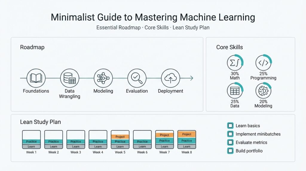
Building on this foundation, think of our approach as a compact machine learning roadmap that focuses on the core skills you actually use in production and a lean study plan for rapid mastery. Start by identifying the minimum mathematical tools, coding fluency, and model families you must master to ship results; then align weekly milestones to experiments and deployable artifacts. This orientation keeps learning outcome-driven: every concept you study should map to a concrete task such as feature engineering, model selection, or deployment automation.
The path splits into clear stages: foundations, applied modeling, productionization, and specialization. Foundations cover linear algebra, probability, and Python data tooling so you can reason about algorithms and implement them from first principles; applied modeling trains you to phrase problems, choose between classical models and neural networks, and evaluate trade-offs; productionization teaches containerization, APIs, and monitoring so models survive the real world; specialization is where you deepen in NLP, computer vision, or time series depending on your product needs. Each stage trains a different mix of theory and practice, and progressing sequentially reduces cognitive overhead while preserving momentum.
A compact twelve-week study plan works well for focused practitioners: week 1–2 for math refresh (matrix ops, eigenvectors, conditional probability), week 3–4 for Python and data pipelines (pandas, vectorized ops, data validation), week 5–6 for classical ML (logistic regression, decision trees, cross-validation), week 7–8 for deep learning fundamentals (backprop, PyTorch/TensorFlow basics), week 9–10 for MLOps basics (Docker, model serving, CI/CD), and week 11–12 for a capstone that includes deployment and observability. How do you prioritize which models to learn first? Prioritize based on the problems you face: tabular prediction first for business analytics, convolutional models for visual tasks, transformers for sequence-heavy work. This pacing balances depth with deliverables so we train skills, not just knowledge.
In daily practice, adopt a tight experiment loop: define hypothesis, implement a minimal training pipeline, run controlled experiments, and interpret metrics. For example, start with a reproducible training scaffold: dataset -> dataloader -> model -> loss -> optimizer -> train/validate loop, then iterate by changing the feature set or regularization. Including a short code skeleton in your workbench makes hyperparameter sweeps and ablation studies practical, and pairing each experiment with a short README helps you and your team reproduce results later. Real projects rarely need perfect theory; they need fast iterations and reproducible results.
Validation and metrics are non-negotiable skills; they separate guesswork from engineering. Always split data to preserve a held-out test set, use cross-validation for small datasets, and pick metrics aligned to business impact (AUC for ranking, F1 for imbalanced classes, or latency/throughput for production constraints). Track experiments with simple tools—CSV logs or a lightweight tracking server—before you invest in enterprise solutions; the discipline of recording hyperparameters and seed values prevents wasted hours chasing nondeterministic outcomes.
When a model proves its value, production readiness requires different choices than research: containerize the model with Docker, expose a minimal inference API, add health checks, and instrument inputs/outputs for drift detection. Automate deploys with a CI pipeline that runs smoke tests and basic performance checks, and register artifacts in a model registry so you can roll back safely. Observability matters: you need lightweight telemetry (latency, error rates) and periodic data-slice evaluations to detect concept drift before users notice.
Finally, treat this roadmap as an iterative loop rather than a checklist; we sharpen skills by shipping small, meaningful projects, reviewing failures, and then specializing. Contribute to an open-source dataset task, pair on a productionization sprint, or build a single end-to-end demo in two weekends to cement learning. In the next section we’ll drill into the first practical sprint, where we transform a toy dataset into a deployable predictor and prove the whole pipeline end-to-end.
Prerequisites: Math and Coding
Building on this foundation, math and coding are the gatekeepers that let you turn intuition into working machine learning systems. What math and coding skills do you actually need to ship models? You should treat mathematical fluency and programming fluency as paired tools: math gives you the language to reason about models and failure modes, while coding turns those ideas into reproducible pipelines and deployable artifacts. Early investment here reduces wasted experiments and speeds iteration across the whole roadmap we described above.
Start with the minimal set of mathematical concepts that you will use day-to-day: linear algebra, probability and statistics, and the basics of calculus. Linear algebra (vectors, matrices, and eigenvectors) is not abstract—it powers feature representations, PCA, and many tensor shape bugs you’ll debug in production. Probability and conditional probability let you translate business questions into metrics and loss functions (for instance, mapping class-imbalance concerns to proper thresholding or cost-sensitive objectives). Calculus matters practically for optimization: gradients and chain rule are the mechanics behind backprop, so derive a simple logistic regression gradient by hand at least once to see how theory maps to code.
On the coding side, prioritize Python and its scientific stack because they’re the lingua franca of production ML teams. Become fluent with NumPy broadcasting, vectorized operations, and pandas for tabular ETL—these skills buy you orders-of-magnitude speedups over row-wise loops and make experiments deterministic. Implement a reproducible training scaffold (dataset -> dataloader -> model -> loss -> optimizer -> train/validate loop) and use small code patterns that force good hygiene: set random seeds, version your data schema, and lock dependency versions. A short code habit like testing a one-epoch run in CI catches many deployment surprises early.
Integrate math and coding with concrete exercises that map to product tasks. For example, implement logistic regression from scratch using NumPy: compute the linear logits, apply the sigmoid, derive the loss and its gradient, then vectorize the update step. This single exercise solidifies linear algebra, probability (logistic link), numerical stability (log-sum-exp tricks), and coding patterns (batching, shape assertions). Another practical example is implementing PCA for dimensionality reduction and validating it against scikit-learn results; this teaches eigenvectors, reconstruction error, and how to benchmark algorithmic correctness in code.
How should you prioritize study time so it accelerates real work? Focus on problem-driven micro-projects: week-long sprints that each produce a shippable artifact. In week one, refresh matrix ops and implement a linear model; in week two, build a small data pipeline with pandas and unit tests; in week three, run k-fold cross-validation and instrument metrics aligned with product impact. We emphasize doing fewer, deeper projects—implementing models from first principles, then converting them to a standard framework (PyTorch/TF) and finally wrapping inference in a minimal API—because that sequence forces you to confront both theory and engineering trade-offs.
As we move into the first practical sprint, keep one rule: every concept you learn must map to a concrete task you can ship. Math without code leaves gaps; code without math leads to brittle experiments. In the next section we’ll convert a toy dataset into a deployable predictor, so make sure your environment has Python, NumPy, pandas, and a lightweight training scaffold ready—these tools are the bridge between your theoretical understanding and production-ready machine learning.
Core Concepts and Algorithms
Building on this foundation, the practical heart of machine learning is understanding a small set of core concepts and a handful of algorithms you’ll use over and over. We want you to be able to answer a simple question quickly: How do you choose between a linear model, a tree, or a neural network for a production task? Front-loading those choices—model selection, training loop design, and error decomposition—lets you trade experimentation time for reliable outcomes.
Start with representation and error decomposition because they shape every algorithmic decision. Representation means how you map raw inputs into numeric features or embeddings; poor representation creates irreducible error. The bias–variance tradeoff (bias: systematic error; variance: sensitivity to training noise) explains why high-capacity models overfit small datasets while simple models underfit complex patterns. Regularization (explicit penalties or architecture constraints) reduces variance by constraining model capacity; think L2 weight decay for linear models or maximum tree depth for decision forests.
Next, think in terms of algorithm families and when they shine. Linear and generalized linear models are fast, interpretable, and robust when features are predictive after simple transformations—ideal for business tabular tasks where explainability matters. Tree-based algorithms (random forests, gradient boosted trees) excel on heterogeneous features and missing values with minimal tuning. Neural networks scale to high-dimensional and unstructured data (images, audio, text) but demand more data, compute, and careful hyperparameter tuning. Kernel methods and nearest-neighbor approaches are useful for small datasets or similarity-based tasks but don’t scale as well to millions of rows. Use model selection to match the algorithm family to data size, latency budget, and interpretability needs.
Optimization and the training loop are where algorithms become results. Optimization refers to the numerical procedure that minimizes your loss function—stochastic gradient descent (SGD) variants, quasi-Newton methods, and coordinate descent are common examples. A well-structured training loop logs loss, validation metrics, and key system metrics every epoch and includes checkpoints and early stopping. For instance, a compact PyTorch-style loop looks like: for epoch: for batch in loader: pred = model(batch); loss = criterion(pred, target); loss.backward(); optimizer.step(); scheduler.step(); instrumenting that loop with learning-rate schedules and batch-size experiments often yields larger gains than chasing exotic models.
Validation strategy and metrics drive trustworthy comparisons. Always keep a held-out test set for final evaluation and use k-fold cross-validation for small datasets to stabilize estimates. Pick metrics that map to business outcomes: precision/recall or F1 for imbalanced classification, AUC for ranking, RMSE for regression, and latency/throughput for production constraints. Calibrate probability outputs (e.g., Platt scaling) when downstream decisions depend on reliable probabilities rather than just rankings.
Controlling capacity and preventing overfit is an engineering practice as much as a mathematical one. Regularization techniques vary by model: L1 promotes sparsity in linear models, dropout and batch-norm affect neural network generalization, and column subsampling reduces correlation in tree ensembles. Ensembling (bagging or stacking) trades compute for robustness; ensembles often win on benchmarks but increase inference cost. Measure throughput and memory footprint as part of algorithm selection so you don’t ship a model that can’t meet operational budgets.
When we evaluate trade-offs, prioritize deployability alongside raw accuracy. Model selection must include latency, retrain frequency, explainability, and maintenance overhead—trees are easier to explain and faster to serve in many cases, neural nets may require GPU inference and more sophisticated observability. Feature stability matters: features that drift frequently require simpler models or automated retraining pipelines. Ask yourself: what is the worst-case failure mode, and how quickly can we detect and roll back?
Taken together, these concepts form a practical toolkit: map problem → choose algorithm family → design training loop → validate with aligned metrics → control capacity → assess deployability. In the next hands-on sprint we’ll transform this theory into a reproducible experiment: a minimal training artifact you can run, measure, and iterate on while keeping observability and deployment constraints front and center.
Practical Data Workflows
Building on this foundation, the hardest part of shipping reliable models is not the algorithm but the plumbing that feeds them: a resilient data pipeline and strict data validation at every stage. We start by treating your data pipeline as a first-class artifact—versioned, tested, and observable—so you can reason about failures the same way you reason about model bugs. How do you build a data pipeline that remains robust as feature sets and team size grow? The short answer is to enforce immutability, schema contracts, and incremental validation from ingest to feature store.
Design your pipeline around clear stages and responsibilities so each step has a single purpose. Ingest raw sources into an immutable landing zone, perform deterministic cleaning and normalization in a transform layer, and materialize feature vectors in a feature store or versioned artifact repository; this separation makes feature engineering auditable and reproducible. We prefer pipelines that are idempotent and checkpointed: if an upstream table changes, you should be able to re-run only the affected transforms rather than the whole flow. Explicit schemas and lightweight data catalogs help teams discover what each dataset contains and which transformation produces the canonical feature vector.
Implement practical patterns that scale from prototypes to production without rewriting everything. Start with simple batch jobs for nightly aggregation and a thin streaming layer for near-real-time signals; avoid premature optimization but design the API between layers so you can swap execution engines later. For feature engineering, codify transformations as composable functions with unit tests—one function per transformation reduces coupling and speeds debugging. Store intermediate artifacts with immutable names that include a deterministic hash of upstream inputs; this lets you reproduce any model training by pulling the same feature artifact and seed values.
Make data validation non-negotiable and automate it where possible to catch issues before they reach training runs. Define both structural checks (schema, column types, nullability) and statistical checks (value ranges, cardinality changes, quantile shifts) and fail fast on regressions. Integrate lightweight assertions into CI pipelines so a pull request that changes a transform also runs validation against a small sample dataset; for larger datasets, run sampling-based or summary-stat checks that approximate full scans. Recording validation outputs alongside experiment logs ensures you can trace a performance regression back to a specific data snapshot or transformation.
Operate the pipeline with continuous monitoring and observability so you detect data drift and broken assumptions quickly. Instrument latency, throughput, and row counts at each stage and track feature distributions over time; alert when a key feature’s median or null rate drifts beyond a configurable threshold. Data drift and label skew require different responses—drift in inputs may call for retraining or feature re-engineering, while label shift often signals upstream business changes that need product-level fixes. Automate detection-to-action flows where an alert can create a retraining job, open a ticket, or roll back to a previous feature artifact.
Finally, bake reproducibility and collaboration into your workflow so experiments remain actionable across teams. Record data lineage, feature manifests, and the exact artifact hashes used for training in the model registry and experiment tracker; this reduces ambiguity when you need to debug production failures or audit a decision. Treat the data pipeline as code: review transformations in PRs, run unit and integration tests, and include short README documentation for each dataset. Taking these steps turns feature engineering and data preparation from fragile one-off tasks into predictable, maintainable engineering work that scales as your models move from prototype to production.
Model Evaluation and Tuning
Model evaluation and hyperparameter tuning drive the difference between a toy model and a production-ready predictor; if you neglect them, you ship brittle behavior instead of reliable software. In the first 100 words we’re prioritizing the core mechanics: model evaluation, cross-validation, metrics, and hyperparameter tuning. Treat evaluation as an engineering discipline: it answers whether a model will generalize, what kinds of errors it makes in the wild, and which knobs materially change performance under production constraints. If you approach tuning like an academic exercise you’ll waste compute and time—approach it like debugging a system instead.
Building on this foundation, your validation strategy should be explicit and reproducible. Use a held-out test set for final, untouchable estimates and rely on cross-validation (k-fold CV, where the dataset is partitioned into k disjoint folds and each fold is used once as a validation set) or stratified splits when data are imbalanced. For time-series or causally ordered data, replace random folds with time-based splits to avoid leakage from future to past. Define and fix these splits before any modeling or feature selection so that every experiment is comparable and we avoid optimistic bias.
Pick metrics that map directly to product impact rather than chasing a single accuracy number. How do you pick the right metric? Ask: what decision follows from the prediction? Use AUC or mean average precision for ranking problems, precision/recall or F1 when false positives and false negatives have asymmetric costs, RMSE or MAE for regression tasks tied to dollar loss, and latency/throughput for operational constraints. Also evaluate calibration (probability reliability) when downstream logic uses predicted probabilities; a calibrated model can be the difference between profitable automation and costly errors.
Hyperparameter tuning is a search problem over model configuration rather than model architecture. A hyperparameter is any setting that isn’t learned during training (learning rate, regularization strength, tree depth, batch size). Start by tuning the most influential hyperparameters—learning rate, weight decay, and tree depth—before fine-grained sweeps. Use simple strategies first: random search often outperforms grid search for the same compute budget, and early-stopping reduces wasted evaluations. If you need more sophistication, adopt Bayesian optimization or population-based training, but only after you’ve stabilized preprocessing and your validation protocol.
Diagnostics complement metrics: they tell you why a model succeeds or fails. Plot learning curves (training vs validation error versus dataset size) to detect high variance or persistent bias, inspect confusion matrices for class-specific failure modes, and use residual plots for regression. For feature-level insights, compute feature importance and use model-agnostic tools like SHAP values to find unexpected correlations or spurious signals. These analyses guide meaningful interventions—collect more data, add regularization, or engineer a small, stable feature set—rather than blind hyperparameter chasing.
Make your evaluation robust to common pitfalls. Guard against data leakage by ensuring preprocessing steps that compute statistics (scalers, encoders) are fit only on training data within each fold. For hyperparameter selection, use nested cross-validation or keep a separate validation set to avoid optimistic tuning bias. Consider the operational trade-offs of ensembling: ensembles often improve held-out performance but increase inference cost and observability complexity. Measure inference latency, memory footprint, and retrain frequency as first-class evaluation metrics.
Instrument the experiment loop so results are auditable and reproducible. Log dataset hashes, seed values, hyperparameters, model artifacts, and evaluation metrics into an experiment tracker or even structured CSVs when you’re starting. Version feature artifacts and record the exact validation split used for each run; this makes regressions diagnosable and rollbacks safe. Small discipline here—consistent logging, short experiment READMEs, and deterministic pipelines—saves hours when you later compare a tuned model against a simpler baseline.
Next, we’ll apply these principles in a hands-on sprint where we run controlled cross-validation, tune a compact set of hyperparameters, and practice the diagnostic steps that reveal practical failure modes. That session will translate evaluation results into concrete changes—feature edits, retraining triggers, or deployment-safe ensembles—so we move from measured experiments to reliable production behavior.
Lean Study Plan
Most engineers treating machine learning as a skill want results, not a catalog of concepts—so we design a study plan that privileges outputs over hours. Start by committing to a concrete, outcome-driven artifact for each short sprint: a validated model, a runnable inference endpoint, or a reproducible experiment report. This front-loaded focus accelerates learning and supports rapid mastery because every study session maps to an engineering deliverable you can test and iterate on.
The core principle is minimal viable mastery: pick the smallest piece of the stack that will teach the largest set of skills and ship it. That means pairing a tight theoretical target (for instance, understanding gradient descent behavior on a logistic loss) with an engineering task (implement the optimizer, run an ablation, and log stability under different seeds). Deliberate practice—short, focused exercises with immediate feedback—beats long passive reading; when you practice a pattern like feature validation, model training, or CI smoke tests, you internalize both the why and the how.
Structure your weekly rhythm around two-hour deep-work blocks and a single end-of-week demo. In a typical weekday, spend the first block on learning or algorithm derivation, the second block on code (data ingestion, transformation, or a one-epoch sanity run), and reserve an hour for instrumentation and notes. Timebox exploratory activities: limit a hyperparameter sweep to a fixed compute budget and aim to reach a decision (keep, tune, or discard) by the end of the block. We find this mix of study and application enforces discipline and keeps the study plan measurable and repeatable.
Make each mini-sprint deliverable-focused so you can evaluate progress without re-reading notebooks. For example, a two-week mini-sprint might target a production-ready tabular classifier: week A proves data quality with automated checks and a k-fold baseline; week B improves a candidate model, wraps it in a lightweight inference API, and runs basic latency and throughput tests. Deliverables are explicit: a dataset manifest with hashes, a validation report answering “what breaks on a cold start?”, a reproducible training script, and an endpoint with health checks. Those artifacts let you iterate with confidence and hand off work to teammates.
Keep reproducibility and lightweight tracking non-negotiable from day one. Record dataset hashes, random seeds, exact preprocessing steps, and the commit hash that built the artifact; store these in a small run README or a structured CSV if you’re not yet using a tracking server. Reproducible artifacts reduce repeated debugging and let us compare experiments as we tune models. When you run into nondeterministic behavior, this minimal checklist usually points you to the culprit—data shuffle, floating-point differences, or a leaking preprocessing step—faster than guessing.
How do you know when to move on from a line of investigation? Treat learning curves and marginal gains as your decision criteria: if additional model complexity yields diminishing returns on your primary product metric or increases inference cost beyond the operational budget, stop and shift focus. Similarly, prefer data collection when error analysis shows systematic patterns that models can’t learn, and prefer simpler models when explainability or latency matters. These decision points keep the study plan lean and aligned with product impact rather than academic curiosity.
Finally, fold retrospection into your cadence so each sprint improves the next one. After every demo, write a two-paragraph retrospective: what worked, what failed, and a single prioritized next step. That habit closes the learning loop, turns ad-hoc experiments into institutional knowledge, and sets up the next sprint’s objective. Building on what we’ve practiced so far, our next hands-on session will convert one of these mini-sprints into a complete end-to-end demo you can run and iterate on together.