Overview and Objectives
Building on this foundation, we frame why a production-ready evaluation system matters for modern LLM development: experiments without rigorous tracking are noisy, non-reproducible, and hard to scale. Native LLM Evaluation needs to live where your data and compute already are, so you can compare model outputs against large, versioned datasets with minimal ETL. By colocating evaluation inside Snowflake and adopting an MLflow-style approach to runs, artifacts, and metrics, we avoid brittle pipelines and reduce the gap between research experiments and operational validation. This reduces context-switching for engineers and accelerates iteration on prompt design, model selection, and post-processing rules.
The principal objective is to make evaluation first-class and auditable. We want reproducible model metrics stored as immutable artifacts, reproducible prompts and seeds captured per run, and traceability from a metric back to the exact dataset, prompt template, and model version. To achieve this, the system must capture deterministic inputs (prompts, examples, random seeds), the executed model identifier, and the evaluation code or SQL that computed each metric. When you can answer “which dataset, prompt, and scoring function produced this F1?” in a single query, you dramatically reduce debugging time and stakeholder friction.
Scalability and operational cost control are equally critical objectives. Evaluations often require thousands to millions of prompt-model calls and expensive embedding or similarity computations; therefore, we design for parallelized execution using Snowflake’s compute scaling, batching requests to model endpoints, and leveraging vectorized SQL where possible. This approach lets us run embarrassingly parallel workloads across many micro-batches while retaining a central canonical store for results. The MLflow-style log model lets teams compare runs side-by-side, filter by tags (experiment, task, dataset slice), and aggregate metrics across runs without copying large output tables across systems.
We also prioritize extensibility and observability so the framework stays useful as models and objectives evolve. That means modular scoring functions (accuracy, BLEU, ROUGE, embedding-based retrieval metrics, human-in-the-loop labels) implemented as SQL UDFs or stored procedures alongside registration of metric definitions. When the scoring logic changes, we version the metric implementation and tie it to runs; consequently, you can re-evaluate past runs deterministically. For governance and validation, we record result provenance (who ran it, when, compute size, cost estimate) so you can enforce review gates for models that will reach production.
Practically, you’ll instrument evaluations the way you instrument training: register a run, execute, and record artifacts. For example, a minimal flow inside Snowflake can look like this in pseudo-SQL and procedural steps: create a run row in eval.runs, write prompt + outputs to eval.outputs, compute metrics with eval.compute_metrics(run_id), and persist aggregated metrics to eval.metrics_summary. The same pattern supports human labeling queues, asynchronous scoring tasks, and backfills. By treating evaluation runs as first-class objects you can reproduce a result by replaying the run’s inputs and metric code against the same snapshot of the dataset.
Moving forward, the important consequence is that evaluation becomes action-oriented: you can trigger automatic model gating, generate audit reports, or schedule periodic re-evaluations against fresh data slices. How do you ensure reproducible model metrics at scale? By combining Snowflake’s data governance and compute elasticity with an MLflow-style metadata model and clear versioning for prompts and scoring logic. In the next section we’ll map these objectives to concrete schema choices, task orchestration patterns, and cost-aware execution strategies so you can implement a scalable, reproducible evaluation pipeline in your environment.
Architecture and Components
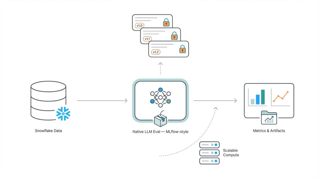
Colocating evaluation metadata and compute inside Snowflake changes the trade-offs for LLM evaluation from “how do we move data” to “how do we instrument runs.” In the architecture we describe, Snowflake becomes the canonical store for prompts, model outputs, and run metadata so you can query and compare experiments without expensive ETL. That MLflow-style approach—registering runs, artifacts, and metrics—lets teams reason about reproducibility and cost in the same place they store labeled data. By front-loading LLM evaluation and reproducible metrics inside your data platform, you reduce context-switching and make auditability a first-class property of every experiment.
At the center of the system is a small set of components that map directly to developer workflows: a runs registry, an outputs store, a metrics registry, and compute primitives that execute scoring logic. The runs registry records deterministic inputs (prompt templates, examples, seeds), model identifiers, and configuration tags so you can reproduce any execution. The outputs store contains raw model responses and intermediate artifacts such as embeddings or token-level alignments. The metrics registry holds versioned metric definitions and links to the SQL UDFs (user-defined functions) or stored procedures that implement them, enabling you to run a single query to compute scores for a given run and metric version.
Execution follows a predictable, parallelizable data flow: snapshot the dataset, materialize prompt micro-batches, call the model (via an external function or batched API worker), persist outputs, then compute metrics with vectorized SQL. For example, a minimal replay is a few SQL steps: insert a row into eval.runs, stream prompts into eval.outputs, then run eval.compute_metrics(run_id). Because Snowflake supports parallel execution and scaling, we batch model calls and push as much work as possible into set-oriented SQL to exploit compute elasticity. This design turns millions of prompt-model calls into an embarrassingly parallel workload while keeping results queryable and auditable.
Versioning and provenance are non-negotiable: every prompt template, metric implementation, and model identifier must be immutable for a given run. We record references to versioned code (commit hash or UDF version), model artifact IDs, and the dataset snapshot used for evaluation. In practice you can combine Snowflake features such as time-travel or zero-copy cloning to preserve the exact table state you scored against, then attach that snapshot to the run row. That way, when you audit a surprising F1 or BLEU, you can trace it deterministically back to the dataset, the prompt, the metric SQL, and the model version that produced it.
Observability and operational controls close the loop: we surface run-level metadata (cost estimate, compute size, executor logs) so you can enforce review gates and schedule re-evaluations on slices that matter. We also integrate human-in-the-loop queues for ambiguous examples and expose tagging so you can filter evaluation runs by task, dataset slice, or prompt family. How do you ensure reproducible model metrics at scale? By making reproducible metrics and MLflow-style run primitives the primitives of your evaluation system, leveraging Snowflake for governance and compute, and instrumenting cost and provenance so that replays, audits, and automatic gating become routine. In the next section we’ll translate these components into concrete schema designs and orchestration patterns you can implement immediately.
Set Up Snowflake Environment
Building on this foundation, get your Snowflake account ready as the canonical execution plane for reproducible LLM evaluation, MLflow-style run tracking, and versioned metrics. Snowflake should be where your runs registry, outputs store, and metrics registry live, so front-load environment setup around security, compute, and schema. By configuring roles, resource monitors, and a dedicated evaluation warehouse up front, you reduce friction when you scale thousands or millions of prompt calls and keep cost and provenance visible from the first run.
Start with governance and access control as a priority because evaluation data is sensitive and audit requirements are non-negotiable. Create a least-privilege role hierarchy for engineers, automation (CI/CD) accounts, and reviewers; assign object ownership to a controlled schema such as eval and use masking policies on PII or proprietary prompts. Configure time-travel retention or zero-copy cloning policies to preserve dataset snapshots referenced by runs so you can reproduce results later, and attach resource monitors to prevent runaway spend during large replays.
Next, provision compute intentionally to balance throughput and cost—this is how you make LLM evaluation practical at scale. Create one or more warehouses sized for parallelized micro-batches and enable auto-resume and auto-suspend to avoid idle charges. Consider multi-cluster warehouses or multiple smaller warehouses when you need concurrent backfills versus a single large run; you can also reserve a small interactive warehouse for governance queries. How do you size for thousands of API-backed prompt calls? Start with a small test cluster and measure round-trip latency per micro-batch, then scale warehouse size and cluster count to match desired throughput while watching resource monitor alerts.
Define a compact, versioned schema that maps directly to the MLflow-style primitives we described earlier: runs registry, outputs store, and metrics registry. Keep records immutable where possible and use Snowflake types that capture flexible metadata—VARIANT for tags, STRING for model identifiers, and TIMESTAMP_LTZ for event ordering. For example, a minimal runs table might look like this:
CREATE TABLE eval.runs (
  run_id STRING PRIMARY KEY,
  created_at TIMESTAMP_LTZ DEFAULT CURRENT_TIMESTAMP(),
  model_id STRING,
  prompt_template STRING,
  seed INTEGER,
  dataset_snapshot STRING,
  tags VARIANT,
  commit_hash STRING
);
Persist raw outputs and embeddings in separate, append-only tables and partition them by run_id and micro_batch_id so you can replay or re-score slices without moving data. Use clustering keys on high-cardinality columns you’ll filter by (task, slice, run_id) to improve compute efficiency for metric aggregation.
Integrate model invocation with Snowflake using the mechanism that fits your security posture—external functions for managed API calls or Snowpark-driven workers that batch requests externally and stream results back. Store API credentials in a secrets manager and reference them via a narrow API integration rather than embedding tokens in SQL. Batch prompts into micro-batches, insert them into eval.outputs, and perform idempotent upserts so retries and partial failures are easy to reconcile. This pattern keeps the heavy network I/O outside set-oriented SQL while keeping the canonical outputs inside Snowflake for metric computation.
Finally, instrument provenance and observability into every object you create so metrics remain auditable and reproducible. Record commit hashes or UDF versions alongside metric definitions, link runs to the exact dataset_snapshot string (or time-travel pointer), and persist execution metadata such as warehouse used, cost estimate, and executor logs. Version metric implementations as stored procedures or UDFs and reference the implementation identifier in your metrics registry so you can re-run old runs against the exact scoring function when needed.
With the environment secured, sized, and modeled this way, we can map those design goals into concrete schema choices, orchestration patterns, and cost-aware execution strategies next. That mapping will show how to implement parallelized scoring, versioned metrics, and gated model promotion using the Snowflake primitives you’ve just provisioned.
Define Tracking Schema and Metrics
Tracking schema decisions are the foundation that make reproducible metrics actionable rather than just data noise. When you design a tracking schema inside Snowflake with an MLflow-style mindset, you prioritize immutable run metadata, explicit links to metric implementations, and per-example outputs that let you reconstruct every aggregate. What should you record per run to make metrics reproducible? At minimum capture the model identifier, prompt template version, dataset snapshot pointer, random seeds, executor metadata (warehouse, cost estimate), and the metric implementation id — these fields let you answer “which code produced this score?” without leaving the data platform.
Building on this foundation, structure the schema around four canonical objects: runs, outputs, metric_definitions, and metric_results. The runs table is your single source of truth for an execution; outputs hold raw responses and per-example scores; metric_definitions version the scoring logic; and metric_results store aggregated, query-friendly summaries. Keep metric_definitions compact but explicit — include a metric_id, human-friendly name, parameter schema, and an implementation reference (commit hash or UDF version). For example:
CREATE TABLE eval.metric_definitions (
  metric_id STRING PRIMARY KEY,
  name STRING,
  impl_ref STRING,
  params VARIANT,
  version INTEGER,
  created_at TIMESTAMP_LTZ
);
Design outputs and metrics so you can compute both per-example diagnostics and roll-ups without re-running model calls. Persist per-example rows with run_id, input_id, model_output, embedding (if used), and per-metric raw_score so you can inspect outliers and diagnose failure modes. Then compute aggregations into a metrics_summary table partitioned by run_id, metric_id, and slice_tag; this separation keeps expensive storage of raw tokens distinct from lightweight dashboards that read aggregated metrics. Use clustering keys on run_id and slice_tag to accelerate queries and keep compute costs predictable when computing metrics at scale.
Versioning metric implementations is non-negotiable for reproducible metrics and auditability. Record an impl_ref that points to a stored procedure version, SQL UDF name plus version, or a commit hash in your repo; include this impl_ref on every metric_result row so replays are deterministic. When you update scoring logic (e.g., change tokenization, add normalization, or switch similarity thresholds), increment the metric_definition version and keep the old impl_ref available so you can re-evaluate historical runs against the new or old logic. This pattern gives you the ability to answer governance questions such as “did this F1 change because the model changed or because the scoring function changed?”
Capture slicing, parameters, and statistical context as first-class fields so filtering and automated gating become simple SQL queries. Store metric parameters (top_k, threshold, similarity_model_id) in the metric_results row and attach slice tags for demographic or task-based partitions; also persist confidence intervals or p-values for A/B comparisons when applicable. This makes it straightforward to build gating queries like SELECT run_id, metric_id FROM eval.metrics_summary WHERE metric_id=’mrr@k’ AND slice_tag=’edge_cases’ AND lower_bound > threshold. By keeping these details in the tracking schema you enable cost-efficient dashboards and automated policy rules without recomputation of raw outputs.
Operationally, plan for two read patterns: deep dives that scan eval.outputs for debugging and fast comparisons that read eval.metrics_summary for dashboards and gating. Materialize common roll-ups and keep per-example output tables append-only and immutable for reproducibility; then use scheduled recompute jobs to backfill metrics when you intentionally change implementations. Taking this approach within Snowflake and adopting an MLflow-style tracking schema ensures your metrics are auditable, reproducible, and actionable — next we’ll map those schema choices into concrete orchestration patterns and cost-aware execution strategies you can implement immediately.
Orchestrate Scalable LLM Evaluations
Building on this foundation, the practical challenge is turning the MLflow-style primitives you already created into a resilient orchestration layer that runs scalable LLM evaluations reliably and cost-effectively in Snowflake. We treat runs as stateful objects and design an executor pattern that moves work through predictable phases: prepare (snapshot + prompt materialization), execute (batched model calls), persist (append outputs), score (vectorized metric computation), and finalize (aggregate summaries and record cost). By front-loading keywords like scalable LLM evaluations, Snowflake, and MLflow-style in your orchestration design, you make it simple to query run status, cost, and provenance from one place and automate downstream gating and reporting.
Start by modeling a run lifecycle with explicit states and micro-batch checkpoints so you can parallelize safely. For each run we create micro-batches with deterministic IDs and insert them into an append-only staging table; workers pick up only batches with a claimed lease token so concurrency is explicit and idempotent. This pattern keeps heavy network I/O outside set-oriented SQL while ensuring you can resume or replay failed batches without duplicating outputs; when a worker finishes a batch it writes a completion marker and cost estimate back to the runs registry so we always know progress at the run_id level.
Parallelization and cost control come from batching, warehouse sizing, and backpressure. Batch prompts to fit your latency/throughput trade-off—larger batches reduce per-request overhead but increase the blast radius of failures—then match micro-batch size to a warehouse cluster configuration that you can autoscale for short bursts. Use resource monitors and a lightweight scheduler that caps concurrent workers per run to avoid runaway spend; we recommend exposing an estimated_cost field on run rows so policy engines can either approve large runs automatically or gate them for manual review.
Design for failures: idempotency, retries, and dead-letter handling are non-negotiable at scale. Use idempotency keys tied to (run_id, micro_batch_id) for each external model call and persist both success and error payloads; transient API errors should be retried with exponential backoff while non-transient failures route the micro-batch to a dead-letter queue for human triage. For partial scoring failures, persist partial metric fragments so you can compute approximate results quickly and replay the remainder later; this strategy reduces mean time to insight while maintaining reproducibility.
Make observability and gating part of the orchestration loop rather than an afterthought. Emit structured telemetry—per-batch latency, token counts, cost, and per-example diagnostic flags—into a materialized metrics_summary that your CI/CD or policy engine can query. Then attach automated gates that query the metrics_summary: if a run’s safety metric or edge-case F1 falls below threshold, fail promotion automatically and create a human review ticket, or route specific examples to a labeling queue for manual adjudication. This tight feedback loop turns evaluation from a reporting task into an operational control point.
Finally, plan for re-evaluation and reproducible replays as core capabilities of the orchestrator. Each run must reference immutable pointers—dataset snapshot, prompt_template version, and metric impl_ref—so you can re-run scoring on demand when you update a metric implementation or want to measure drift against fresh data. Schedule periodic re-evaluations for production models using the same orchestration primitives (snapshot, micro-batch, execute, score), and keep a separate backfill queue for intentional recomputes so they don’t contend with interactive governance queries. By building orchestration that treats runs, metrics, and provenance as first-class citizens inside Snowflake, we make scalable LLM evaluations auditable, repeatable, and operationally useful for real-world model governance and deployment workflows.
Visualize, Export, and Reproduce
Snowflake should be the first word in your mental model when you think about turning ad-hoc LLM checks into reproducible metrics and MLflow-style evaluation artifacts. We want reproducible metrics that are not only queryable but also visualized, exported, and replayed without leaving the data plane. This section shows how to turn the runs, outputs, and metric_definitions you already store into dashboards, portable artifacts, and deterministic replays so teams can answer questions like “How do you prove a dropped F1 was caused by a model change and not a scoring tweak?” while keeping auditability central to the workflow.
Start with visualization as a data-first activity: build your dashboards directly on eval.metrics_summary and slice-tagged roll-ups so every chart answers a reproducibility question. Create time-series charts that plot metric_id by run_id and overlay impl_ref or commit_hash as an annotation to expose scoring-function drift; link those charts to drill-down queries that select from eval.outputs for failing examples. For interactive debugging, design a small set of parameterized views (for example, a view that filters by slice_tag, model_id, and metric_version) so you can pivot from an aggregate KPI to concrete examples with two clicks, and ensure your visualization layer can accept VARIANT or JSON parameters to reproduce the exact filtering used in the run.
Exporting artifacts should be treated as a first-class step in every run lifecycle so you can hand off reproducible artifacts to reviewers, compliance teams, or downstream systems. Persist a canonical export that includes the run row, the dataset_snapshot identifier, the prompt_template version, and the outputs table slice for that run; serialize these into a compact format such as newline-delimited JSON for per-example records and Parquet for columnar analytics. Use Snowflake’s COPY INTO to stage those artifacts to cloud storage and include a manifest file that lists impl_ref, commit_hash, and the time-travel pointer used; this manifest is what auditors query to verify that an exported metric came from the exact code and snapshot you claim.
Reproducing a run should be a deterministic, two-step operation: restore or reference the exact dataset snapshot, then re-run the metric implementation referenced by impl_ref. In practice that means attaching the run’s dataset_snapshot to your session (or creating a zero-copy clone for an isolated replay), inserting the recorded prompts back into eval.outputs if needed, and executing the stored procedure or SQL UDF whose name and version are stored in metric_definitions. Because every metric_result row contains the impl_ref and metric parameters, we can re-evaluate historical outputs against a new impl_ref or re-run the original impl_ref against a fresh snapshot to measure drift—both operations are simple SQL transactions that produce auditable, reproducible outputs.
You’ll also want visual artifacts that make reproductions obvious and actionable: include per-example diff views, token-level alignment highlights, and embedding-similarity heatmaps so reviewers can see exactly which examples changed and why. How do you validate whether a metric delta is statistical noise or a meaningful regression? Produce confidence intervals and sample-size metadata as part of the exported summary and display them prominently in the dashboard; combine those with automated annotations (impl_ref changes, prompt edits, model version bumps) so your visualizations tell the reproducibility story at a glance. Embedding visualizations and per-example links into the same UI that surfaced the aggregate metric reduces the turnaround time from discovery to root-cause to remediation.
Finally, operationalize visualization, export, and replay as part of your orchestrator rather than ad-hoc tasks: emit an export step on run completion, trigger automated snapshots and COPY INTO jobs, and record the export manifest in eval.runs so gating logic can pick it up. Schedule periodic replays against fresh data slices using the same MLflow-style primitives (snapshot, micro-batch, compute_metrics) and surface those replay results in the same dashboards used for interactive inspection. By coupling visualization with reproducible exports and deterministic replays inside Snowflake, we close the loop between insight and audit, making evaluation an operational control rather than a manual audit task.