NLP Overview and Scope
Natural Language Processing (NLP) sits at the intersection of linguistics, statistics, and software engineering, and it’s the set of techniques we use to turn human language into actionable signals for machines. In the next few paragraphs we’ll map the practical territory: common tasks, typical architectures, and engineering trade-offs you’ll meet when building production systems that require robust machine understanding. This overview primes you to decide when to reuse a pretrained model, when to annotate a dataset, and when to invest in a retrieval layer for accuracy and provenance.
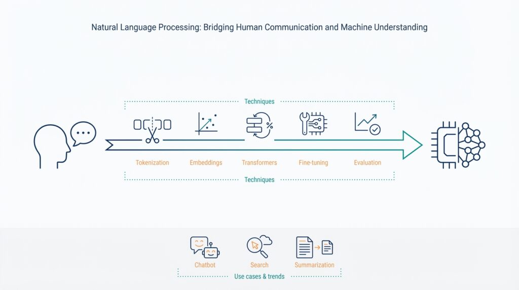
At its core, the field groups around a small set of repeatable tasks that solve most business needs. Text classification assigns discrete labels (spam vs. not-spam); named entity recognition (NER) extracts structured entities like dates or product names; sequence-to-sequence models handle translation and summarization; question answering and retrieval combine to answer factual queries; and token-level tasks (tokenization, part-of-speech tagging) prepare text for downstream models. When we mention terms like tokenization or embedding, we mean the low-level transformations that make text machine-readable: tokenization splits raw text into units, and embeddings map those units into numeric vectors that capture semantic relationships.
Different algorithmic approaches dominate different parts of the stack, and choosing the right one matters. Historically, rule-based systems and feature-engineered classifiers handled many problems, but statistical methods and neural architectures—especially transformer-based language models—now lead due to their generalization and pretraining benefits. A transformer models relationships across tokens using self-attention, which makes it effective for long-range dependencies; contrast this with RNNs that lost traction for many production tasks. For practical engineering, we often combine approaches: a lightweight classifier for intent routing, a transformer for contextual understanding, and rules or heuristics for high-precision edge cases.
Engineering an NLP pipeline is as much about data and evaluation as it is about model choice. Begin by defining success with concrete metrics: is latency more important than F1? Do you need exact matches (precision) or broad coverage (recall)? Use domain-specific test sets for validation, and measure both intrinsic metrics (F1, BLEU, ROUGE) and extrinsic business metrics (task completion rate, user satisfaction). Preprocessing choices—normalization, subword tokenization, handling of out-of-vocabulary terms—often change outcomes more than swapping model architectures, so instrument those transformations and version your preprocessing pipeline along with model checkpoints.
We encounter these decisions in real systems every day. For an intent-classification service, we might start with a few hundred labeled examples, spin up AutoModelForSequenceClassification from a pretrained checkpoint, and fine-tune for a few epochs; for enterprise document search, we’ll use embeddings plus a vector database and apply retrieval-augmented generation (RAG) to ground answers in source documents. How do you choose between fine-tuning and a prompt-based approach? Use fine-tuning when you have labeled, domain-specific data and need deterministic behavior; use prompt engineering or few-shot techniques when data is scarce and iteration speed matters. Also plan for model monitoring: drift detection, confidence calibration, and human-in-the-loop workflows for continuous improvement.
Building on this foundation, the scope of applied NLP includes not just model training but data strategy, deployment patterns, and governance. You’ll need CI/CD for models, rollout strategies (canary, shadow), privacy-preserving techniques for sensitive text, and a taxonomy for bias mitigation and auditing. As we move to concrete techniques and case studies next, keep those operational constraints top-of-mind—your choice of architecture should optimize for maintainability, observability, and alignment with product goals rather than raw benchmark performance.
Text Preprocessing and Tokenization
Preprocessing is the most influential change you can make before touching model architecture; small token-level decisions often shift downstream F1 and retrieval quality more than swapping a transformer checkpoint. We start by treating preprocessing and tokenization as an engineering contract: every transformation you apply to training data must be identically applied at inference. That means logging the tokenizer version, normalization rules, and any heuristics (like URL masking or de-identification) alongside model artifacts so you can reproduce behavior and diagnose drift without guessing which step changed.
Normalization choices shape the signal your model learns, so decide them with downstream tasks in mind. Apply Unicode normalization and consistent whitespace handling to remove noisy duplicates, but be cautious about aggressive lowercasing if you rely on casing for entity detection; preserving case often improves NER and intent detection in domain-specific systems. Consider selective cleaning — for example, normalize punctuation and strip control characters for chat logs but retain punctuation and formatting for code or log-parsing tasks — because overly broad cleaning can erase task-relevant features.
Tokenizers come in many flavors and each has trade-offs: whitespace and rule-based tokenizers are fast and transparent; subword methods like BPE, WordPiece, and unigram models compress vocabulary size and gracefully handle out-of-vocabulary (OOV) words. Subword tokenization generally wins for cross-domain and morphologically rich languages because it balances vocabulary size and expressiveness, but it introduces label-alignment complexity for token-level supervision. How do you choose between whitespace tokenization and subword models for a domain-specific corpus? Use whitespace for extremely constrained grammars or when you need exact token alignment, and choose subword tokenizers when you expect high lexical variety or need compact embedding matrices.
Practical implementation favors using a stable tokenizer API with explicit parameters for special tokens, unknown-token handling, truncation, and padding. For example, instantiate a pretrained tokenizer, fix max-length behavior, and serialize the tokenizer files with your model:
from transformers import AutoTokenizer
tok = AutoTokenizer.from_pretrained("my-checkpoint")
ids = tok("AcmeCorp paid $1,200 on 2025-03-12.", truncation=True, max_length=128)
Set truncate/pad policies to match downstream batching and record whether you applied post-tokenization filters (like removing tokens below a frequency threshold) because those change embedding indices and break old checkpoints.
Real-world edge cases force pragmatic choices: multilingual pipelines need language detection before tokenization or a language-unified tokenizer like SentencePiece; noisy user text benefits from spelling normalization or byte-level models; domain-specific terms (drug codes, product SKUs, code snippets) often justify a custom vocabulary built from in-domain corpora. For token-level tasks such as NER, explicitly map token pieces back to original labels using rules (first-piece labeling, BIO propagation) and validate with a label-alignment test suite to avoid subtle label drift during training and inference.
Operationally, treat preprocessing as part of your model’s API surface: version everything, include deterministic RNG seeds for any stochastic normalization, and run unit tests that assert identical token sequences for stored example inputs. Monitor token distribution drift in production—changes in token frequencies are an early signal of domain drift that warrants retraining or tokenizer refresh. Taking these steps ensures your token representations remain stable, interpretable, and maintainable as we move into embedding strategies and model selection in the next section.
Language Representations and Embeddings
When you move from tokenization to anything that actually powers understanding, embeddings become the glue that turns discrete text into navigable geometry. Building on this foundation, we treat language representations as vectors that capture semantics, syntax, and usage patterns so downstream systems — search, clustering, classification, or RAG — can operate in a continuous space. This matters for both retrieval latency and model accuracy: well-designed embeddings let you trade off dimensionality and compute for real-world gains in semantic search and intent resolution. How do you choose the right representation for your use case and constraints?
Start by distinguishing static vectors from contextual embeddings. A static embedding assigns one vector per word or token regardless of context; a contextual embedding produces different vectors depending on surrounding text (for example, “bank” in a financial vs. river sentence). Static vectors are compact and fast for large vocabularies, but they fail when polysemy or sentence-level meaning matters. Contextual embeddings from transformer encoders give you richer sentence- or token-level signals that improve downstream tasks like question answering, paraphrase detection, and NER alignment.
In practice, generate and normalize embeddings deterministically so your production pipeline is reproducible. For sentence-level vectors we often use a pooled output from a pretrained encoder and then L2-normalize before indexing; for token-level tasks you can average subword vectors or apply attention-based pooling to preserve salient spans. For example, a minimal PyTorch pattern looks like this:
# pseudo-code
tok = tokenizer(text, return_tensors="pt", truncation=True)
out = model(**tok).last_hidden_state
vec = out[:,0,:].detach()          # CLS pooling or mean over tokens
vec = vec / vec.norm(dim=1, keepdim=True)
This deterministic flow — tokenization, model checkpoint, pooling rule, and normalization — must be recorded in the same way you version tokenizers and preprocessing earlier. Small changes in pooling or truncation will move vectors in embedding space and break nearest-neighbor behavior, so include unit tests that assert stable distances for canonical examples.
After you have vectors, a vector database becomes the operational layer for scale and latency. Insert normalized vectors with metadata, then perform approximate nearest neighbor queries for semantic search and retrieval-augmented generation. In production you’ll pick an index type (HNSW, IVF+PQ, etc.) based on throughput and memory: dense indexes favor recall, quantized indexes save RAM but trade accuracy, and batched k-NN queries improve GPU throughput for low-latency requirements. Use cosine similarity for angle-based semantics when vectors are normalized, or dot product when you’ve trained with that objective — mismatch between training loss and index metric is a common source of poor retrieval quality.
Decide when to fine-tune embeddings versus using off-the-shelf models by weighing labeled data, domain vocabulary, and maintenance costs. Fine-tuning or contrastive-training on in-domain pairs gives you sharper cluster boundaries for product catalogs, legal text, or medical records, but requires curated positives/negatives and CI for safety and bias checks. If you lack labels, use prompt augmentation, weak supervision, or create synthetic pairs from existing KB relations to bootstrap targeted embeddings that outperform general-purpose checkpoints on domain-specific retrieval tasks.
Operational monitoring must include embedding-specific signals: distributional drift in vector norms, degradation of nearest-neighbor recall on a validation set, and rising query-document distance for frequent queries. Regularly recompute embedding-centroid stability and run adversarial checks (typos, code snippets, multilingual noise) because embeddings are sensitive to preprocessing changes in ways that classifier logits are not. Also track privacy and bias: embeddings can leak demographic signals, so audit similarity behavior across sensitive groups and apply differential privacy or filtering when necessary.
Taking these practices together, we treat representations and embeddings as an engineered interface between language and application logic — not a fixed artifact. Next, we’ll connect this layer to retrieval and grounding strategies so you can build search and generation systems that are both precise and explainable.
Transformer Models and Fine-tuning
Transformer architectures revolutionized NLP by making large-scale pretraining and targeted fine-tuning practical; when you combine a pretrained model with task-specific data, you get dramatic accuracy improvements with comparatively little labeled data. This approach—transfer learning using transformer checkpoints—front-loads linguistic and world knowledge into model weights so your downstream classifier or generator starts from a strong prior instead of from random initialization. Building on our earlier discussion of tokenization and embeddings, fine-tuning changes how those contextual representations map to task labels, so small engineering choices during adaptation have outsized effects on performance and stability.
Start by picking the right adaptation strategy for your constraints: full fine-tuning, partial freezing, or parameter-efficient methods like adapters and LoRA. Full fine-tuning updates every weight and often yields the best accuracy for large labeled sets, but it increases storage and rollback complexity because each task requires a full checkpoint. Freezing lower layers and training only the top blocks or a classification head reduces compute and stabilizes optimization, and discriminative learning rates (lower for early layers, higher for task-specific layers) help when you mix general-language and domain-specific signals. How do you decide which path to take? Use the size and quality of your labeled data, latency and deployment constraints, and maintenance budget as primary signals.
When you have limited labels or strict deployment limits, parameter-efficient fine-tuning (PEFT) is often the right trade-off. Adapters inject small task-specific modules into each transformer block; LoRA (low-rank adaptation) constrains weight updates to low-rank matrices, dramatically reducing the number of trainable parameters and the size of saved artifacts. These approaches let you keep a single base pretrained model in production while swapping tiny adapter files per task, which simplifies CI/CD and A/B testing and lowers storage and inference compatibility issues across teams. For retrieval and embedding alignment, contrastive fine-tuning of the encoder (training with in-domain positive/negative pairs) sharpens nearest-neighbor clusters without touching decoder weights.
Practical training details matter as much as model choice: control your learning rate schedule, batch size, and gradient accumulation to avoid catastrophic forgetting and unstable loss spikes. Use a low initial learning rate (often 1e-5—5e-5 for transformers) with warmup steps and cosine or linear decay; apply weight decay and layer-wise learning-rate decay for regularization when fine-tuning large checkpoints. Mix precision (FP16) and gradient checkpointing to reduce memory pressure; validate with a held-out set for early stopping rather than relying solely on training loss. For sequence labeling tasks like NER, ensure your tokenization-to-label alignment is deterministic (first-piece labeling or BIO propagation) because subword splits can silently corrupt metrics if not handled consistently.
A minimal Hugging Face pattern for supervised fine-tuning illustrates the workflow and reproducibility checklist: tokenize with the same tokenizer used for pretraining, record pooling/aggregation rules for embeddings, and fix seeds for determinism. Example (Trainer API pattern):
from transformers import AutoTokenizer, AutoModelForSequenceClassification, Trainer, TrainingArguments
tok = AutoTokenizer.from_pretrained("my-checkpoint")
model = AutoModelForSequenceClassification.from_pretrained("my-checkpoint", num_labels=3)
args = TrainingArguments("out", per_device_train_batch_size=16, learning_rate=2e-5, num_train_epochs=3)
# prepare datasets with tok(..., truncation=True, max_length=128)
trainer = Trainer(model=model, args=args, train_dataset=train_ds, eval_dataset=dev_ds)
trainer.train()
After you ship a fine-tuned model, monitor both accuracy and distributional signals: calibration, confidence drift, embedding-centroid shifts, and production latency. Run adversarial and domain-shift tests (typos, mixed language, unusual punctuation) and track per-query degradation in nearest-neighbor recall if you fine-tuned embeddings. Finally, version adapters or LoRA deltas separately from the base pretrained model, adopt shadow testing or canary rollouts for new checkpoints, and automate rollback triggers based on business metrics as well as validation loss—those operational practices keep fine-tuning from becoming a maintenance liability as your product evolves.
Popular Use Cases and Applications
Building on this foundation, the most visible value of NLP in production comes from solving concrete business workflows where text is the primary signal: customer support, knowledge discovery, compliance, and automation. In these areas, embeddings and semantic search power retrieval that feels human—matching intent rather than exact keywords—and they show up early in the architecture when you need high-recall search across documents, tickets, or product catalogs. We’ll show practical patterns you can adopt, explain trade-offs between retrieval-augmented generation (RAG) and direct generation, and outline when fine-tuning a transformer beats prompt engineering.
Customer-facing conversational systems are one of the highest-impact use cases for NLP because they directly change user experience and operational cost. Start by routing intents with a light classifier, then escalate to a contextual generator for long-form answers; combine intent classification with named entity recognition to extract structured fields for ticket creation or routing. In practice, teams deploy a hybrid pipeline: a fast intent model for routing, an embedding-based semantic search for relevant knowledge snippets, and a generator conditioned on those snippets to produce an answer with citations. This pattern reduces hallucination and keeps latency predictable.
Enterprise search and knowledge discovery are where embeddings and vector indexes deliver measurable ROI: legal teams, support engineers, and product managers need semantic search that surfaces conceptually related documents even when queries use different vocabulary. Implement sentence-level embeddings for chunked documents, index with HNSW or IVF+PQ depending on memory and throughput, and normalize vectors for cosine-based retrieval consistency. How do you evaluate quality? Use domain-specific recall tests and measure downstream task success (time-to-resolution, number of follow-ups) rather than generic similarity scores.
Document understanding—contracts, invoices, and medical records—combines extraction, classification, and grounding. Here, token-level models (NER, span-prediction) extract structured facts and embeddings link those facts to canonical records or ontologies for reconciliation. For example, extract parties and dates with a fine-tuned sequence-labeling head, then compute embeddings for clause-level similarity to find precedent clauses across a corpus. This two-stage approach (extract then retrieve) keeps extraction precise while leveraging semantic search to surface context and precedents.
Generative summarization and automated content generation are valuable when you need concise, readable outputs from long inputs: meeting notes, legal briefs, or research literature. Use a retrieval step to gather salient passages, then feed them into a conditioned generator to produce summaries that cite sources. If you have labeled summaries, prefer supervised fine-tuning; when labels are scarce, use prompt templates plus few-shot examples and control generation with constrained decoding or reranking using embeddings to measure fidelity to source texts.
Question answering and RAG are essential when users ask specific queries over an internal knowledge base or document store. RAG systems combine retrieval with generation so answers are grounded, which improves trust and auditability compared to unconstrained generation. If you need deterministic, high-precision answers (billing rules, regulatory text), fine-tune a model on QA pairs and keep a retrieval layer for provenance; if speed of iteration is more important, prototype with prompt-based RAG and iterate on retrieval and chunking strategies.
Operational and safety-focused applications include content moderation, PII detection, and bias auditing—areas where you must instrument performance and failure modes. Use embeddings to detect semantic drift (query-document distance increases), monitor calibration for classifiers, and implement human-in-the-loop review workflows for edge cases. Also version your tokenizer, embedding pipeline, and retrieval index as part of the model contract so changes in preprocessing don’t silently break production behavior.
Taken together, these applications show how NLP translates to business impact: semantic search and embeddings unlock discovery, extraction and NER enable structured automation, and RAG plus fine-tuning give you grounded generative capabilities. As we move to deployment patterns and observability, we’ll apply these use cases to concrete CI/CD strategies and rollback criteria so you can ship robust language systems without sacrificing explainability or maintainability.
Deployment, Evaluation, and Ethics
Building on this foundation, deployment, evaluation, and ethics are the operational trinity that determines whether an NLP system becomes useful—or dangerous—in production. We deploy models with an eye toward reproducibility, observability, and rollback semantics so you can iterate rapidly without compromising user trust. Early in the pipeline, define service-level objectives (SLOs) for latency and accuracy, and record the exact tokenizer, checkpoint, and preprocessing contract that accompanies every release; these artifacts are the reference for future audits and debugging. Why do these choices matter? Because deployment decisions shape how you detect failures, run evaluations, and enforce ethical safeguards at runtime.
Start your deployment strategy by treating models as first-class software artifacts: versioned checkpoints, serialized tokenizers, and small adapter deltas must travel through CI/CD just like code. Use staged rollouts—shadowing and canary releases—so new checkpoints process a subset of live traffic while writing full telemetry; this lets you validate both model quality and operational characteristics under real-world distributions without impacting all users. For low-latency services, container orchestration and autoscaling policies should reflect the model’s memory and GPU requirements, and we recommend separate inference paths for heavy RAG-style generators versus fast intent classifiers to keep tail latency predictable. When you design deployment pipelines, include automated sanity checks that reject artifacts if basic invariants (tokenizer mismatch, output shape, or size) fail.
Evaluation must marry offline rigor with online business metrics: intrinsic metrics (F1, BLEU, ROUGE) tell you about model behavior on curated test sets, while extrinsic metrics (task completion rate, time-to-resolution, escalation rate) measure customer impact. How do you decide when to roll back a model? Define concrete rollback triggers ahead of time—statistical drops in business KPIs, sudden calibration shifts, or increases in error rates on golden queries—and automate rollbacks for high-risk thresholds while keeping a human-in-the-loop for nuanced decisions. Slice-based evaluation is critical: evaluate by language, query intent, document type, and confidence bands so you can find brittle subpopulations that aggregate metrics hide. Also validate calibration (reliability diagrams, temperature scaling) and threshold policies for gating automated decisions.
Robust test-and-release pipelines include adversarial and stress testing. Run typo and code-snippet tests, mixed-language and domain-shift scenarios, and hallucination checks for generative components by comparing generated claims against a provenance layer. For systems using retrieval-augmented generation, enforce grounding tests that measure citation fidelity and insert provenance checks that make it trivial to trace answers back to original documents. We run red-team exercises and synthetic attack suites to surface prompt-injection or data-poisoning risks before wider release because pre-production adversarial failures are far cheaper to fix than post-production incidents.
Monitoring and observability close the loop between deployment and evaluation: instrument latency, tokenization errors, confidence distributions, embedding-centroid drift, and nearest-neighbor recall on a rolling validation set. Alert on distributional changes—shifts in token frequency, spike in unknown-token rates, or drift in embedding norms—because these early signals often precede accuracy degradation. Log sufficient metadata (input hash, tokenizer version, model delta id, retrieval document ids) to support reproducible incident investigation and compliance audits, and expose model-level metrics alongside business KPIs in dashboards so teams can correlate technical regressions with user impact.
Ethics is not a checkbox; it’s an operational discipline we bake into every stage of the pipeline. Perform regular bias audits across sensitive attributes using fairness metrics appropriate to your task, maintain data provenance and consent logs for sensitive corpora, and apply privacy controls—PII detection, redaction, or differential privacy—where required by policy. Document decisions in model cards and datasheets so downstream teams understand limitations and intended use-cases, and keep human review workflows for high-risk predictions. Finally, make transparency a runtime property: when answers rely on retrieved documents or potentially sensitive inferences, surface provenance and confidence so users and auditors can judge the output.
Operationalizing these practices gives you reliable deployment velocity, defensible evaluation, and measurable ethical controls that scale with product complexity. Next we’ll apply these operational patterns to CI/CD templates and monitoring playbooks so you can automate the muscle memory that keeps models safe, debuggable, and aligned with user expectations.