What Is Language Modeling
Building on this foundation, language modeling is where we teach a system to guess what comes next in a sequence of words. How do you train a machine to do that? In practice, a language model assigns a probability to the next word and, by extension, to an entire sentence, so it can rank likely continuations instead of producing one rigid answer. That is why autocomplete, speech recognition, and many modern text systems all lean on language modeling: they are really playing a prediction game one word at a time.
To make that prediction possible, the model studies a training corpus, which is simply a large collection of text used for learning. Think of it like reading thousands of recipe books before trying to guess the next ingredient in a new recipe: you are not memorizing one dish, you are learning patterns. When the model sees a fragment like ‘I packed my suitcase with’, it can assign higher probability to words such as ‘clothes’ or ‘shoes’ than to a random word like ‘elephant’, because the text patterns in the corpus make those continuations more plausible. The important idea is not human-like understanding; it is probability based on experience, and that experience comes from text the model has already seen.
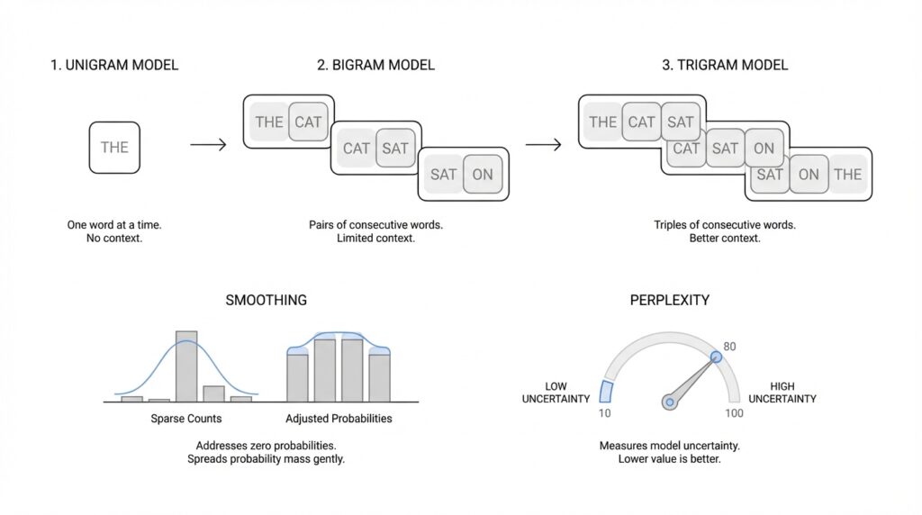
This is where n-gram language models enter the story. An n-gram is a sequence of n words, and the n-gram model uses only a short recent window rather than the whole conversation, which is a simplifying Markov assumption, meaning we pretend the recent past carries most of the useful information. A unigram looks at one word at a time, a bigram looks at the previous word, and a trigram looks at the previous two words. That limited view sounds modest, but it gives us a practical way to estimate probabilities from counts and to see how much context actually helps when we model language.
Of course, real language is messy, and that is where smoothing comes in. If a word sequence never appeared in training, a raw count-based model can hand it a probability of zero, which is like telling the system that a perfectly normal sentence is impossible. Smoothing is the safety net: it redistributes a little probability mass so unseen or rare events still get a chance, often by blending counts from simpler evidence or by backing off to a smaller context. This is one of those quiet but crucial ideas in language modeling, because it keeps the model from collapsing the moment it meets something unfamiliar.
Once the model is built, we need a way to ask whether it is actually doing a good job, and perplexity gives us that check. Perplexity measures how surprised the model is by an unseen test set, which is a dataset we held back from training, and lower perplexity means the model is assigning higher probability to the text it has not seen before. In plain language, a model with lower perplexity feels less confused by real text and more confident about the next word. That is why perplexity is so useful in language modeling: it turns a vague sense of ‘this seems better’ into a number we can compare, and it prepares us for the next step, where unigram, bigram, and trigram models become different ways of choosing how much context to trust.
Unigram Models Explained
Building on this foundation, the unigram model is the simplest place to start in language modeling, and that is exactly why it is so useful. If you have ever wondered, “How do you teach a machine to guess words without giving it much context?” a unigram model is the first answer we reach for. It treats each word as if it can be judged on its own, like looking at individual ingredients before thinking about a full recipe. In a language model, that means we estimate how likely each word is by counting how often it appears in a training corpus, which is the large collection of text we use for learning.
The idea is refreshingly plain: more common words get higher probability, and rarer words get lower probability. If a corpus contains “the” thousands of times and “zebra” only a few times, the unigram model will naturally favor “the” because it has seen it more often. This is one reason unigram language modeling feels so approachable for beginners, because it turns text into a simple frequency table. We are not asking the model to understand grammar, meaning, or word order yet; we are only asking it to learn which words tend to show up most often.
That simplicity is both the strength and the limitation of the unigram model. On one hand, it is easy to build, easy to explain, and fast to compute, which makes it a helpful baseline when we begin comparing language models. On the other hand, it ignores context entirely, so it cannot tell whether a word makes sense in the sentence around it. A unigram model might know that “coffee” is common, but it cannot tell whether “I spilled my coffee” is more natural than “I spilled my rain,” because it does not look at neighboring words.
Still, the unigram model teaches us something important about language modeling: probability starts with evidence. Each word receives a probability based on its share of the total word counts, and all those probabilities add up to 1 across the vocabulary, which is the full set of words the model knows about. Think of it like dividing a pie among all the words in the training data; the biggest slices go to the words that appear most often. This is where unigram language modeling becomes a stepping stone, because once you understand how counts turn into probabilities, it becomes much easier to see why bigger models need more context.
A unigram model is also a good reminder that “better than nothing” can still be valuable. In tasks like rough text generation, basic classification, or as a benchmark for more advanced methods, the unigram model gives us a clean starting point. If a more complex model cannot beat this simple baseline, then something is wrong or the added complexity is not helping yet. That is why people still talk about unigram models in NLP: they are small, but they set the bar.
There is also a practical lesson hiding inside this simple approach. When we build a unigram language model, we learn how sparse data, rare words, and probability estimates interact before we add the complications of word order. That makes it easier to appreciate why the next step, bigrams, matters so much: once we let one neighboring word influence the prediction, the model begins to move from word frequency toward actual sentence structure. And that shift, from isolated words to word pairs, is where the story of context really starts to unfold.
Bigram And Trigram Models
Building on this foundation, bigram and trigram models are where language modeling starts to feel less like word counting and more like listening to short fragments of speech. Instead of asking, “How common is this word on its own?” we begin asking, “What word usually comes next after the one, or two, words we just saw?” That small change matters a lot, because it gives the model a sense of context, and context is what makes language feel natural. A bigram language model looks at one previous word, while a trigram model looks at the previous two words.
A bigram model works like a careful reader who keeps only one word of memory. If the model sees “I want,” it can estimate that “to” is a strong next word because that pair appears often in the training corpus, which is the large collection of text used for learning. In other words, the model does not treat every word equally anymore; it learns that some word pairs travel together more often than others. This is the heart of bigram language models: we count how often a word follows another word, then turn those counts into probabilities.
Once you see that idea, the trigram model feels like the next step in the same story. Now the model remembers two previous words instead of one, so it can make a more specific guess about what comes next. For example, after “I want to,” the word “go” may feel more likely than it did after only “to,” because the extra word sharpens the pattern. How do you make a language model sound more fluent? You usually give it a little more context, and the trigram model does exactly that by capturing short phrases and common word sequences.
This extra context is powerful, but it also introduces a tradeoff that beginners notice quickly. The more words we ask the model to remember, the more specific the pattern becomes, and the harder it is to find that exact pattern in the training data. A bigram language model might see “strong coffee” often enough to make a confident guess, while a trigram model might struggle if it rarely sees the full three-word sequence around that phrase. So while trigrams can feel smarter, they also face a bigger data sparsity problem, which means many useful word combinations appear too rarely to estimate cleanly.
That is why smoothing becomes so important here. When a bigram or trigram model encounters a sequence it has never seen, it cannot treat that sequence as impossible, because real language keeps inventing new combinations all the time. Instead of relying on raw counts alone, we soften those estimates and allow the model to borrow a little confidence from shorter patterns. This helps the model stay usable when the text becomes unfamiliar, and it prevents the language model from sounding overly brittle. In practice, smoothing is what keeps bigram and trigram models from falling apart the moment the training data gets thin.
You can think of the difference between these models as the difference between reading with a flashlight and reading with a wider beam. A unigram model sees one word at a time, a bigram model sees a word plus its immediate neighbor, and a trigram model sees a slightly wider slice of the sentence. That wider slice often helps the model choose better continuations, especially for fixed expressions and common grammar patterns, which is why n-gram language models became such a useful stepping stone in NLP. They are simple enough to understand, but rich enough to show how context changes prediction.
As we move forward, the main lesson to keep in mind is this: bigrams and trigrams do not try to understand language the way people do. They learn local patterns and use those patterns to make the next-word guess feel more grounded. The moment you let a model look at neighboring words, it stops guessing from pure frequency and starts using sentence structure, which is exactly the bridge we need before we talk about how to measure whether those guesses are actually any good.
Why Smoothing Fixes Sparsity
Building on this foundation, smoothing is the step that keeps n-gram language models from getting stuck when the text runs thin. If you have ever asked, Why does a model fail on a perfectly normal sentence?, the answer is often sparsity, which means the training corpus does not contain enough examples of every possible word sequence. In plain language, the model has seen many things, but not everything it might face later. Smoothing fixes that gap by making the model less brittle and more willing to cope with unfamiliar text.
The problem starts with raw counts. In a bigram or trigram language model, we estimate the next word from how often a sequence appears in the training data, and that works well until a sequence never appears at all. Then the model may assign it zero probability, which is like saying, “This sentence can never happen.” That is far too harsh, because real language constantly produces new combinations, and even common phrases can be missing from a limited corpus. Once a model gives zero probability to one unseen piece, the whole sentence probability can collapse to zero as well.
This is where smoothing earns its place. Think of it like sharing a small emergency fund across all the words the model might need to guess. Instead of giving every observed sequence all the credit and every unseen sequence none, smoothing nudges a little probability mass toward rare or unseen events. That tiny adjustment does not pretend we know more than we do; it simply admits that the training data is incomplete and gives the model room to breathe.
That idea becomes especially important as context gets longer. A unigram model only tracks single words, but bigrams and trigrams need exact word pairs or triples, and those are much rarer in any corpus. As we discussed earlier, the more context you add, the more specific the pattern becomes, and the more likely it is to go missing. Smoothing helps n-gram language models survive that sparsity by borrowing confidence from shorter patterns when the longer one is too thin to trust. So instead of acting as if “I want to” is the only phrase that matters, the model can still lean on “want to” or even “to” when needed.
Another helpful way to see it is to imagine a recipe book with missing pages. If your favorite recipe skips a step, you do not throw the whole dish away; you use nearby clues, familiar techniques, and the broader cooking pattern to fill the gap. Smoothing works the same way. It may back off to a smaller n-gram, which means it falls back from a trigram to a bigram or from a bigram to a unigram when the longer sequence is too rare. That backup plan keeps the model useful even when the exact phrase has never shown up before.
This is also why smoothing improves learning, not just prediction. A model trained without smoothing can become overconfident in the data it has seen and too harsh about everything else. A smoothed language model is more balanced, because it treats rare events as possible instead of impossible, and that makes its probability estimates more realistic. In practice, that means better generalization: the model handles new sentences, odd phrasing, and out-of-vocabulary-like patterns with much less panic. How do you make a language model less fragile? You give it a way to be uncertain in a controlled, mathematically sensible way.
Once that clicks, the big picture becomes clearer. Sparsity is not a bug in language itself; it is a natural result of finite training data meeting an almost endless space of possible word combinations. Smoothing is the bridge between those two realities, letting the model stay grounded in evidence without being trapped by missing counts. That is why, in n-gram language modeling, smoothing is not a small adjustment tacked on at the end. It is the quiet mechanism that turns raw frequency counting into something that can actually face real language.
Measuring Perplexity
Building on this foundation, perplexity is the moment when a language model stops being a clever guesser in theory and gets put on the spot in practice. When we ask how to measure perplexity, we are really asking a simple question: how surprised is the model when it meets new text it did not train on? That matters because a model can sound impressive on paper, yet still stumble when it faces real sentences. Perplexity gives us a way to turn that gut feeling into a number we can compare.
To measure it, we first hold out a test set, which is a set of text we keep separate from training so the model cannot memorize it ahead of time. Think of it like studying flashcards at home and then taking a quiz with new questions from a different deck. The model reads each word in that unseen text and assigns a probability to what comes next, and perplexity summarizes those probabilities across the whole test set. In plain language, a low perplexity score means the model was less startled by the text, while a high score means it kept guessing awkwardly or with low confidence.
Here is where the idea becomes especially useful: perplexity is not about whether the model got every word exactly right. Instead, it asks whether the model gave reasonable probability to the words that actually appeared. If the model keeps assigning high probability to the correct next words, its perplexity drops. If it spreads its confidence too thin or leans toward unlikely words, perplexity rises. That is why perplexity in language modeling feels a bit like reading the model’s level of uncertainty out loud; it tells us how well the model’s internal expectations match real language.
A helpful way to picture this is to imagine two students taking the same fill-in-the-blank quiz. One student has read widely and can usually predict the missing word from context, while the other keeps reaching for strange answers. The first student would have lower perplexity because the test text rarely catches them off guard. The second student would have higher perplexity because the quiz feels more confusing at every step. So when people ask, “Why does perplexity matter?” the answer is that it gives us a fair, repeatable way to judge how confidently a model handles new text.
Perplexity also helps us compare models that use different amounts of context. Earlier, we saw that unigram, bigram, and trigram models each look at different windows of text, and perplexity tells us which one handles unseen sentences more gracefully. A model with better context use often earns lower perplexity, but only if it also manages sparsity well, which is why smoothing still matters here. Without smoothing, even a good model can be unfairly punished by rare or unseen word combinations, and its perplexity can shoot up for reasons that have more to do with missing data than with true language skill.
One detail that often confuses beginners is that perplexity is a relative score, not a universal badge of intelligence. A value of 20 does not mean the model is “20 percent good” or that it only has 20 possible choices in its head. It means the model is, in a sense, as uncertain as if it had to pick among about 20 equally likely options at each step. That is why perplexity is most useful when we compare models on the same dataset, under the same conditions, rather than treating the number as meaningful all by itself.
If you want to remember one practical idea, remember this: perplexity measures how well a language model predicts what comes next on text it has never seen before. It rewards models that assign sensible probabilities and punishes models that are overly surprised by ordinary language. That makes it one of the clearest ways to tell whether our unigram, bigram, or trigram model is moving in the right direction, and it sets us up to compare these models with confidence as we move forward.