Token Classification Overview
Building on this foundation, token classification is where the model starts placing a label on every token in a sentence. How do you turn a sentence into labels? We first split the text into tokens, which are the word-like pieces the model reads, and then assign a category to each one. In practice, that means one token can be marked as part of a person, a location, a verb, or the start of a phrase. Hugging Face describes token classification as classifying each token in a sequence, and it points to NER and POS tagging as the most common examples.
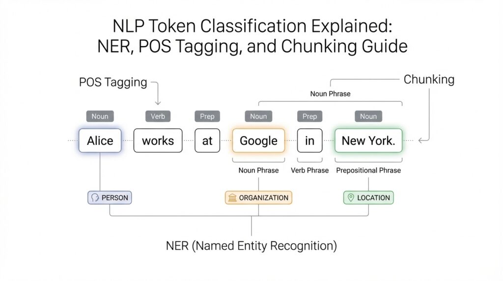
Once you see it that way, NER, POS tagging, and chunking feel less like separate mysteries and more like three versions of the same game. NER, or Named Entity Recognition, looks for real-world names such as people, places, and organizations; the common B- and I- labels mark the beginning and inside of an entity span. POS tagging, or part-of-speech tagging, gives each token a grammatical role such as noun or verb. Chunking, sometimes called chunk parsing, groups tokens into non-overlapping phrases like base noun phrases. The labels differ, but the rhythm is the same: read the sentence, then label each token with enough detail to rebuild meaning.
This is where context matters. A single word can wear different hats depending on the sentence around it, so token classification leans on neighboring words instead of judging each token in isolation. SpaCy’s tagger, for example, is a trainable pipeline component that predicts part-of-speech tags, and its pipeline shows how those tags feed later processing steps. That same idea helps the model decide whether a token is part of a name, a verb phrase, or the boundary of a chunk. Think of it like a chef tasting the whole soup before deciding which spice is missing; one ingredient alone rarely tells the whole story.
When you look at the output, the pattern becomes easier to read. Each token gets a label, and those labels together tell you what the sentence contains: who is mentioned, what kind of words appear, and which neighboring tokens belong together. In NER, that might let you pull out New York City as one location instead of three separate words; in chunking, it might let you spot a noun phrase; in POS tagging, it might show that a word is functioning as a noun rather than a verb. Hugging Face’s task guide and task summary both frame token classification this way, and the examples make clear that the model is doing structured annotation, not freeform generation.
That is the mental model to keep as we move forward: token classification is sequence labeling with a purpose. Instead of asking the model for one answer for the whole sentence, we ask it to annotate every token, and that annotation becomes the raw material for NER, POS tagging, and chunking. Once that clicks, the rest of the topic starts to feel far less abstract, because the outputs are not mysterious scores but a neatly labeled map of the sentence. With that map in mind, we can now look at how those labels are encoded and learned.
NER, POS, and Chunking
Building on this foundation, the easiest way to think about NER, POS tagging, and chunking is that they are three different lenses for reading the same sentence. Named entity recognition, or NER, asks, “Which words point to real-world things like people, places, or companies?” Part-of-speech tagging, or POS tagging, asks, “What job is each word doing in the sentence?” Chunking asks, “Which neighboring words belong together as a phrase?” When you first meet token classification, these can feel like separate puzzles, but they are really variations of the same careful labeling game.
What makes NER especially useful is that it turns scattered words into meaningful units. If a sentence contains “San Francisco Bay Area,” NER tries to treat that as one location span instead of three unrelated tokens floating by themselves. That matters because real text is messy: names can stretch across multiple words, abbreviations can hide inside larger names, and a single token can be ambiguous on its own. In practice, NER helps you pull useful facts out of text, whether you are scanning customer messages, news articles, or support tickets. It is one of the clearest examples of token classification doing real work.
POS tagging works differently, because it is less about identifying things in the world and more about understanding grammar. A word like “book” can be a noun or a verb, and the surrounding words are what reveal its role. That is why POS tagging feels a bit like watching an actor change costume depending on the scene. In one sentence, a token may be a noun; in another, the same token may become a verb or adjective. Once the model assigns part-of-speech labels, you can see how the sentence is built, which is useful for parsing, text analysis, and many downstream language tasks.
Chunking sits between those two ideas, almost like the bridge that connects grammar to meaning. Instead of labeling every possible phrase structure, chunking groups tokens into smaller non-overlapping pieces such as noun phrases or verb phrases. Think of it like putting beads into small strands before arranging the whole necklace. You are not building the entire grammar tree yet; you are gathering nearby tokens that clearly belong together. This is why chunking often feels easier to read than a full parse, while still giving you a stronger picture of sentence structure than isolated token labels alone.
How do you know which task you are looking at when the outputs seem so similar? The answer is in the label set and the question the model is trying to answer. NER labels usually point to categories like person, organization, or location. POS tagging labels point to grammatical roles like noun, verb, or adjective. Chunking labels point to phrase boundaries, often using tags that mark where a chunk starts and ends. The structure is the same, but the purpose changes. That is why token classification can support very different kinds of analysis without changing its basic rhythm.
Once these differences click, the practical value becomes much easier to see. NER helps you extract facts, POS tagging helps you understand how words function, and chunking helps you group related words into readable units. Together, they turn a sentence from a flat string into a mapped landscape, where every token has a place and every phrase has a shape. This is the real strength of token classification: it gives you a labeled path through language, so the model is not just reading text but organizing it in a way you can use.
BIO Tagging Basics
Building on what we have seen so far, BIO tagging is the little codebook that helps token classification draw clean boundaries around words. When you want a model to mark names, phrases, or other spans inside a sentence, it needs a way to say where something starts, what continues, and what is outside the target entirely. That is where BIO tagging comes in: it stands for Begin, Inside, and Outside, and it gives every token a small but important role. Think of it like placing flags along a trail so you can tell where a route begins, which steps belong to it, and which steps are off to the side.
How do you tell where one entity ends and the next begins? The BIO scheme answers that question with three labels that work together. B marks the first token of a span, I marks any token that continues that same span, and O marks a token that does not belong to any span at all. So if a sentence contains a person’s name or a location, the model does not have to guess where the group starts and stops from scratch every time; BIO tagging gives it a shared rule for drawing those lines. That is especially helpful in token classification, where the goal is not to generate new text but to label each token in a way that stays consistent.
The easiest way to feel this is with a simple example. Imagine the phrase “New York City” inside a sentence. A BIO tagger might label “New” as B-LOC, “York” as I-LOC, and “City” as I-LOC, where LOC means location. The B tells us the span begins at “New,” and the I tags tell us the rest of the location continues through the next tokens. If the sentence also includes words like “visited,” “last,” or “summer,” those would usually receive O because they are outside the location span. This is why BIO tagging is so useful: it turns a messy stretch of text into a readable map.
Once that pattern clicks, you start to see why BIO tagging is so common in named entity recognition, or NER, which looks for people, places, organizations, and similar real-world names. Multi-word entities are the tricky part, because a name is often spread across several tokens, and a model needs a reliable way to keep the pieces together. BIO tagging solves that problem by making the first token special and the following tokens connected. In practice, that means the model can distinguish “San” from “San Francisco,” or “Bank” from “Bank of America,” instead of treating every token as an isolated guess.
There is also a quiet benefit hiding inside the O label. At first glance, O can feel like the least interesting tag, but it is what gives the scheme its breathing room. Without O, every token would have to belong to some span, and that would make ordinary words look more important than they are. By marking the outside tokens clearly, BIO tagging helps the model focus on the exact parts of the sentence that matter for the task. This is one reason sequence labeling feels organized rather than chaotic: the model learns not only what to notice, but also what to ignore.
A helpful way to remember BIO tagging is to compare it to highlighting a paragraph by hand. The B tag is where you first put the highlighter down, the I tags are the rest of the words you keep coloring, and the O tags are the words you leave untouched. That same idea applies whether you are doing named entity recognition, phrase chunking, or another token classification task that needs spans to stay neat. BIO tagging does not make the language simpler, but it makes the model’s decisions easier to read, which is exactly what we want before we move on to more advanced label patterns.
Prepare Labeled Data
Building on this foundation, the next question is practical: how do you prepare labeled data so token classification can learn from it instead of getting confused by it? At this stage, we are no longer talking about sentences in the abstract; we are building the examples the model will study. Think of labeled data as the recipe card for training, where every token needs the right instruction in the right place. If the labels are messy, inconsistent, or misaligned, even a strong model will struggle to learn the pattern you want.
The first step is to decide what each label means before anyone starts annotating. Annotation, which means assigning labels to text by hand, works best when the rules are written down in plain language. For NER, that means agreeing on what counts as a person, organization, or location; for POS tagging, it means deciding how to label nouns, verbs, adjectives, and other parts of speech; for chunking, it means defining which phrases belong together. These rules act like a map, and without them, two people can look at the same sentence and walk away with different answers.
That is why consistency matters so much. If one annotator labels “New York University” as a single organization while another splits it into separate pieces, the model sees conflicting lessons and learns a blur instead of a rule. We often call the process of checking agreement between annotators inter-annotator agreement, which is a measure of how often people make the same labeling choices. When agreement is low, it usually means the instructions are unclear, the label set is too broad, or the edge cases need more discussion. In token classification, a clean label guide is often more valuable than a large but confusing dataset.
Once the labeling rules are stable, the next challenge is aligning labels with the tokenizer, which is the tool that breaks text into tokens. This is where preparation gets a little tricky, because the words humans see are not always the tokens the model sees. A tokenizer may split a word into smaller pieces, called subwords, and your labels must follow that split without losing the original meaning. So if one entity spans several tokens, the labels need to stay attached to the right pieces; otherwise, the model learns a distorted version of the sentence. How do you keep that alignment from slipping? By checking the tokenized output carefully and making sure each original span still maps cleanly to the right labels.
A simple example makes this easier to picture. Suppose you have the phrase “San Francisco Bay Area” in a sentence and you want to mark it as one location. During labeling, you record the full span first, then make sure the tokenized version still carries that same location signal across the correct tokens. If the tokenizer splits a word like “Francisco” into smaller pieces, you still want the label sequence to reflect one continuous entity rather than four unrelated fragments. This is the moment where labeled data stops being a spreadsheet task and starts becoming model training fuel.
Before training begins, it also helps to create a clean split between training, validation, and test data. The training set teaches the model, the validation set helps you tune choices while development is still underway, and the test set gives you a final check on performance. These splits matter because token classification can look strong on the examples it has already seen and weaker on new text from the real world. Keeping the sets separate protects you from fooling yourself with overly optimistic results. It is a small piece of preparation, but it saves a lot of confusion later.
The last pass is quality control, and this is where the dataset starts to feel ready rather than merely collected. We want to spot inconsistent labels, missing spans, duplicate examples, and awkward edge cases before they become training noise. A few careful review rounds often reveal patterns, like repeated mistakes with multi-word names or confusion around punctuation, that are easy to fix once you know where to look. When the labeled data is clean, consistent, and aligned with the tokenizer, token classification has a far better chance of learning the structure you intended. That gives us a solid dataset to work with as we move into how the model actually learns from those labels.
Align Tokens and Labels
Building on this foundation, the real puzzle is not writing labels at all—it is making sure those labels land on the right tokens after tokenization. Human readers see words, but a model often sees smaller pieces called subwords, which are fragments produced by a tokenizer, the tool that breaks text into model-friendly units. That means token classification only works cleanly when the original labels stay in step with the tokenized output. How do you keep a person, place, or phrase attached when one word turns into two or three pieces? That is the alignment problem, and it is one of the quiet details that makes or breaks a training set.
The simplest way to think about alignment is to picture a row of matching stickers. Before tokenization, each word has one sticker. After tokenization, some words need more than one sticker, and some positions get extra markers that do not belong to any word at all. This is common in NER, POS tagging, and chunking, because those tasks label tokens rather than whole sentences. If the tokenizer splits “Washington” into smaller pieces, the label still has to describe the full word or entity, not drift across the sentence like a loose thread. Once you see that, token alignment starts to feel less mysterious and more like careful bookkeeping.
The most common rule is to give the main label to the first token of a word and then handle the later pieces in a consistent way. In named entity recognition, for example, the first subword of “Francisco” might carry the location label, while the remaining subwords either repeat that label or are masked so they do not count separately, depending on the training setup. The important thing is consistency. If one example treats the first subword as the real carrier of meaning and another example spreads the label differently, the model receives mixed signals and learns a fuzzy pattern instead of a sharp one.
Special tokens make alignment trickier, but they are easy to understand once you meet them. Some models add markers such as a start token or an end token to help them process the sequence, and padding tokens are added to make batches the same length. These extra pieces are useful for the model, but they do not belong to the original sentence, so they usually get ignored during loss calculation, which is the process the model uses to measure how wrong its predictions are. In other words, we want the model to learn from real text, not from the scaffolding we used to package it.
This is where word-level and token-level thinking must stay in sync. A word-level label says, “This whole word is a location,” but the model still needs token-level instructions for every piece it actually reads. If you label only the first subword of a split word, you often tell the model to predict on that first piece and ignore the rest. If you label every subword, you must make sure the label scheme supports that choice. The key is not which method you choose, but whether the method matches the rest of your pipeline, from the tokenizer to the training loop to the evaluation script.
A concrete example makes the payoff clear. Suppose the phrase “New York City” appears in a sentence and the tokenizer keeps it as three tokens, or splits one of those words further because of punctuation or casing. A well-aligned dataset still tells the model that all the relevant pieces belong to one location span. That lets token classification behave like a tidy highlighter instead of a confused spotlight, illuminating the whole entity instead of only the first letter of it. The same idea applies in POS tagging and chunking, where the model has to preserve grammatical roles and phrase boundaries even when token boundaries do not match human intuition.
Once alignment clicks, the whole training process feels more trustworthy. You are no longer asking the model to guess where labels should go; you are giving it a sentence map that matches what it actually reads. That careful match between tokens and labels is what turns raw annotations into usable training data, and it is why clean token classification depends as much on preparation as on the model itself. With that bridge in place, we can move forward knowing the labels will follow the text instead of getting lost inside it.
Fine-Tune the Model
Now that the labels are lined up with the right tokens, the model is finally ready to learn from them. This is where fine-tuning enters the story: instead of training a language model from zero, we start with a pretrained model, which is a model that has already learned general language patterns from large amounts of text, and then adapt it to token classification. Think of it like giving a student who already reads fluently a new workbook focused on NER, POS tagging, or chunking. That head start matters, because the model already understands word patterns and only needs to learn the specific labeling rules of your task.
So what does fine-tuning mean in practice? It means we keep training the model on our labeled dataset, but now the goal is narrower and more precise. The model sees each sentence, predicts labels for each token, compares those predictions with the correct answers, and then updates its internal settings to make better guesses next time. That update process is driven by loss, which is a number that tells us how far the prediction is from the truth. When the loss goes down over time, we know the model is learning the shape of the task rather than just staring at the text.
This is also where training choices start to matter in a very human way. An epoch is one full pass through the training data, and a batch is a small group of examples the model learns from at once. If we imagine the data as a stack of flashcards, an epoch is one complete trip through the stack, while a batch is a small handful of cards reviewed together. The learning rate controls how big each update step should be, and that setting can make the difference between careful learning and overshooting the answer. Why does this matter for token classification? Because the model must learn fine details, like where a span begins and ends, without forgetting the broader language patterns it already knows.
A strong fine-tuning run also needs a validation set, which is a separate slice of data used to check progress while training is still happening. This helps us spot overfitting, which means the model is memorizing the training examples instead of learning rules it can use on new text. In NER, POS tagging, and chunking, overfitting often shows up when the model looks impressive on familiar sentences but slips on fresh ones. That is why we watch the validation score, not just the training score, and why we keep an eye on whether the model is improving steadily or getting too confident too fast.
At the end of this process, we usually evaluate token classification with metrics such as precision, recall, and F1 score. Precision tells us how often the model’s predicted labels are correct, recall tells us how many real labels it found, and F1 score balances the two. These metrics are useful because token classification is not only about being right on a few easy tokens; it is about finding the right spans consistently across a sentence. If the model marks “San Francisco Bay Area” as one location, that is a win. If it splits the span incorrectly or misses it entirely, the score reflects that mistake.
Fine-tuning works best when we treat it like careful coaching rather than a one-shot command. We begin with a pretrained model, feed it clean aligned labels, watch how it changes during training, and adjust the settings when it starts drifting. That is the practical heart of token classification: the model is not learning language from scratch, but learning how your particular labeling system works. With that in place, we are ready to look at how to judge the results and understand where the model still gets confused.
Evaluate and Predict
After training, the story shifts from teaching the model to trusting it in the wild. That is where token classification gets its most honest test: how well does it handle new sentences it has never seen before? If you are working with NER, POS tagging, or chunking, the key question is not only did the model learn, but did it learn the right pattern well enough to predict labels on fresh text? Evaluation gives us that answer, and prediction shows us what the model actually does when real language arrives.
Building on the foundation we already set up, evaluation starts with a separate dataset the model never used for training. We check its predictions against the correct labels and measure how often it gets the spans right, not just individual tokens. That distinction matters because token classification is about structure, so a model that marks half of a name correctly has not fully solved the task. For NER, POS tagging, and chunking, the usual lens is precision, recall, and F1 score: precision asks how many predicted labels were correct, recall asks how many true labels were found, and F1 score balances the two into one number.
How do you read those numbers without getting lost? Think of them as three different ways of telling the same story. A model with high precision may be cautious and make few wrong predictions, but it can miss important labels. A model with high recall may catch many real entities or phrase boundaries, but it may also label too much. F1 score helps us compare models more fairly because token classification is usually strongest when it is both accurate and complete, especially when spans matter more than isolated tokens.
While we covered label alignment earlier, evaluation adds another layer: some mistakes are not about the label itself but about the boundary of the span. A predicted location may start one token too early or end one token too late, and that small slip can change the score in a real way. This is why span-level evaluation is so important in NER and chunking, because the model must recover the full phrase, not just recognize a few nearby tokens. In POS tagging, the focus is slightly different, since each token carries its own grammatical role, but the same idea still applies: we want consistent, sensible predictions across the whole sentence.
Now that we know how to judge the model, prediction is where the trained system becomes useful. You feed it a new sentence, the tokenizer breaks that sentence into model-friendly pieces, and the model assigns a label to each token based on what it learned during fine-tuning. Then the labels are decoded back into a human-readable result, so a string of BIO tags becomes a named entity, a part-of-speech sequence, or a set of chunked phrases. This is where token classification stops feeling like a training exercise and starts acting like a tool you can use on emails, articles, support tickets, or any other text stream.
Prediction also reveals why context still matters after training. A word that looked clear during evaluation can become ambiguous in a new sentence, and the model has to rely on nearby words to make the best guess. That is especially true in NER, where a capitalized word might be a person, a place, or something else entirely depending on the sentence. It is also true in POS tagging, where the same token can shift roles, and in chunking, where phrase boundaries depend on the shape of the surrounding words. The model is not memorizing a dictionary; it is reconstructing meaning from patterns.
At this stage, a careful reader should also look beyond the overall score and inspect the mistakes. Did the model miss multi-word entities? Did it confuse locations with organizations? Did it split a phrase at the wrong boundary? Those patterns tell you more than a single metric ever could, because they show where token classification is still fragile. In practice, that kind of error analysis helps you decide whether to collect more examples, tighten your annotation rules, or adjust the way labels are decoded after prediction.
Once you can evaluate the model and read its predictions clearly, the whole workflow comes together. Training gives the model a sense of the task, evaluation tells you whether that sense is reliable, and prediction shows you how the model behaves on real language. That is the point where token classification becomes more than a labeling method: it becomes a repeatable way to turn text into structured information, and that structure is exactly what makes NER, POS tagging, and chunking so valuable in the first place.