Why PostgreSQL indexes matter
If your production queries are dragging and metrics show high I/O and CPU for simple lookups, PostgreSQL indexes are the single most effective lever you can pull to reduce latency and I/O. An index is a separate data structure that lets the database find rows without scanning the entire table, and knowing when to add or avoid an index separates a responsive system from one that struggles under load. We’ll use terms like B-Tree, GIN, GiST, and BRIN throughout, because choosing the correct index type directly influences query planning and execution for slow queries and large datasets.
An index’s core purpose is to narrow the search space for the planner so queries run in sublinear time relative to table size. In PostgreSQL, the planner decides between a sequential scan (reading whole table) and an index scan based on cost estimates; those estimates depend on table statistics and index selectivity. Selectivity measures how many rows match a predicate — high selectivity (few rows) favors an index. Understanding these mechanics helps you diagnose why queries that seem indexable still fall back to sequential scans: often outdated statistics or non-sargable predicates are the root cause.
Indexes come with operational trade-offs that you must manage actively. Each index adds storage overhead and increases write latency because INSERT/UPDATE/DELETE must also update the index; create UNIQUE and covering indexes only where they provide clear read-side wins. Index maintenance tasks—reindexing, VACUUM, and monitoring index bloat—are part of lifecycle work for high-write tables. If you need to build an index without blocking writes, use CREATE INDEX CONCURRENTLY to avoid long locks, and plan maintenance during lower-traffic windows to minimize application impact.
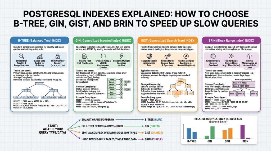
Choosing the right index type matters because different structures optimize different workloads. B-Tree (balanced tree) handles equality and range queries and is the default choice for primary lookups; GIN (Generalized Inverted Index) accelerates full-text search and array containment queries; GiST (Generalized Search Tree) supports nearest-neighbor and spatial queries; BRIN (Block Range INdexes) shines on very large, naturally ordered, append-only tables where index size must be tiny. When should you pick a BRIN over a B-Tree? If your data is physically clustered by the key (for example, time-series logs appended in timestamp order), BRIN delivers orders-of-magnitude smaller index size with acceptable query performance.
You can validate index impact with EXPLAIN ANALYZE, which shows actual runtime and whether the planner used an index-only scan (where PostgreSQL reads the index without fetching heap rows). Build a multi-column index when your queries filter and sort on the same columns — for example, CREATE INDEX ON orders (customer_id, created_at DESC) supports WHERE customer_id = ? ORDER BY created_at DESC LIMIT 20 as an index-only plan if the index contains all needed columns. Also monitor pg_stat_user_indexes and pg_stat_all_tables to detect unused indexes; unused indexes are dead weight for writes and storage.
Building on this foundation, indexing becomes a deliberate design choice rather than a reflexive optimization. We recommend profiling queries, updating statistics with ANALYZE, and experimenting with index types against representative datasets before committing to production changes. In the next section we will examine how B-Tree, GIN, GiST, and BRIN structures differ in memory layout and use-cases so you can match index design to your workload and stop chasing slow queries by guesswork.
B-Tree: ranges and equality
Building on this foundation, B-Tree indexes are the go-to structure when you need fast equality lookups and ordered scans for range queries. B-Tree gives the planner a way to jump directly to matching keys for equality predicates and to walk a contiguous run of index entries for comparisons like >, <, and BETWEEN. In PostgreSQL, that combination makes B-Tree the practical default for primary lookups and for workloads where you filter by an exact key and then page or scan an ordered window.
Equality predicates map cleanly to B-Tree leaf-level lookups: when you write WHERE id = 42 the planner can seek the exact key instead of scanning pages. That seek behavior is why unique and primary-key constraints are implemented with B-Tree by default; you get O(log n) lookup for exact matches. When you use multi-column indexes, remember the left-prefix rule: an index on (a,b,c) supports equality on a, or equality on a and b, but not equality on b alone; design columns so the leftmost column is the one you most frequently test for equality.
Range queries benefit from the B-Tree ordering because the index stores keys in sorted order, enabling the engine to perform an index scan that stops when values leave the requested interval. Queries like WHERE created_at >= ‘2024-01-01’ AND created_at < ‘2025-01-01’ become a single ascending scan over the subset, which is efficient if the interval selectivity is low (few rows). How do you decide whether a range query will use the index? Check selectivity and the estimated cost in EXPLAIN: narrow ranges and predicates that avoid function-wrapping (which breaks sargability) favor index usage.
Here are concrete index patterns that support common equality-plus-range access patterns. Create a composite index when you filter by an equality column and then range on a time or sequence column, and include ordering if you need LIMIT with sort-free results.
CREATE INDEX ON orders (customer_id, created_at DESC);
-- Supports: WHERE customer_id = ? ORDER BY created_at DESC LIMIT 20

CREATE INDEX ON events (user_id, event_time);
-- Supports: WHERE user_id = ? AND event_time BETWEEN ? AND ?
If the query references only indexed columns and the visibility map is up-to-date, PostgreSQL can perform an index-only scan and avoid heap fetches entirely. That makes these composite B-Tree patterns especially valuable for high-throughput read paths where latency and I/O matter.
There are important caveats that change whether B-Tree remains the best choice. If you apply functions to columns (for example, WHERE lower(name) = ‘alice’) you must create a matching expression index; otherwise the planner cannot use the plain B-Tree. Native PostgreSQL range types (int4range, tsrange) expose containment and overlap operators that are usually better served by GiST or SP-GiST indexes rather than B-Tree. Also, very low-selectivity range predicates that match a substantial fraction of the table will often fall back to sequential scans because a full index scan plus heap fetches is costlier than scanning pages sequentially.
In practice, use B-Tree composite indexes to implement cursor-based pagination (WHERE id > last_seen ORDER BY id LIMIT n) and multi-tenant time-window queries (WHERE tenant_id = X AND event_ts >= T1 AND event_ts < T2). Monitor pg_stat_user_indexes and run EXPLAIN ANALYZE to validate that your equality predicates hit the index and that range scans are narrow enough to justify the structure. Keeping statistics fresh with ANALYZE and maintaining the visibility map via VACUUM increases your chances of index-only scans and consistent performance as data grows.
GIN: inverted index for arrays
When your schema exposes multi-valued attributes—tags, roles, or JSON arrays—queries that test containment or membership quickly become the slow path if you rely on sequential scans. GIN (a Generalized Inverted Index) addresses that exact problem by indexing each element inside an array or jsonb document and mapping those elements back to the rows that contain them. By front-loading the keywords GIN, inverted index, and arrays in your query plan, you get a data structure optimized for multi-valued lookups rather than single-key seeks.
The core idea is simple: an inverted index stores a mapping from key (array element, token, or JSON path) to a posting list of row references, rather than storing rows ordered by a single composite key. This makes equality/containment predicates sargable when you ask “does this row contain X?” — for example WHERE tags @> ARRAY[‘payments’] or WHERE data @> ‘{“status”: “active”}’. Because GIN indexes the elements themselves, it supports fast containment and existence queries that would be expensive with a B-Tree, which expects one scalar key per row.
Create a GIN index exactly where your queries test membership or containment. For a tag array you typically write:
CREATE INDEX CONCURRENTLY idx_items_tags ON items USING GIN (tags);
-- Query that benefits:
SELECT id FROM items WHERE tags @> ARRAY['payments'];
For JSONB documents the pattern is identical:
CREATE INDEX CONCURRENTLY idx_docs_data ON docs USING GIN (data);
SELECT id FROM docs WHERE data @> '{"owner_id": 42}';
These examples illustrate how each array element or JSON key/value becomes an index entry, so containment queries become intersection operations over posting lists rather than scans across table pages.
Performance trade-offs matter: GIN indexes are larger and update-costlier than B-Tree because they maintain posting lists for many distinct keys and may keep auxiliary trees for large lists. Writes that insert or remove elements can cause significant index churn, and until the visibility map and vacuuming stabilize the planner may still fetch heap tuples. GIN does offer tunables like fastupdate (which buffers recent inserts) and supports partial indexes to reduce size by limiting indexed rows; use those when write latency or index bloat hits you in production.
How do you decide between a GIN and a B-Tree? Use GIN when your access pattern queries containment, membership, or full-text search across arrays or jsonb objects; prefer B-Tree when you need ordered range scans, equality on a single scalar column, or efficient index-only scans. In practice, we often pair a B-Tree for primary lookups with a GIN for tag/JSON searches. Also consider operator classes: for text pattern search, gin_trgm_ops accelerates LIKE/ILIKE similarity queries, while the default GIN operator class is sufficient for array and jsonb containment.
Apply a few practical rules: test with EXPLAIN ANALYZE against representative data sizes, build GIN indexes CONCURRENTLY to avoid write locks, and use partial or expression GIN indexes when you can constrain or normalize the indexed values to shrink posting lists. For user-facing features like tag filters or permission checks on JSON claims, GIN tends to convert expensive table scans into sub-millisecond lookups. Taking this approach keeps your multi-valued queries efficient as data grows and prepares you to compare GiST or BRIN when spatial or range-oriented patterns become dominant.
GiST: geometric and fulltext
If your queries need proximity searches or geometric intersections, a different index family than B‑Tree will usually save you orders of magnitude in latency. GiST, spatial, and full-text capabilities live in the same general-purpose framework that lets PostgreSQL index complex, non-scalar data types; front-loading those terms helps you decide when to stop relying on table scans and start exploiting indexed spatial or text lookups. In this section we build on the earlier index trade-offs and show how GiST turns geometric containment and some text workloads into indexable operations you can reason about and measure.
GiST is a generalized search tree that stores bounding metadata rather than single scalar keys, which is why it excels for spatial types. The index behaves like an R‑tree variant: each node contains a “bounding box” that summarizes child entries and the planner walks those boxes to eliminate large areas of the search space quickly. That behavior makes GiST ideal for queries that ask “what geometries intersect this polygon?” or “what points lie within this radius?” because the index prunes irrelevant regions without fetching heap rows for every candidate.
Create a GiST index on PostGIS geometry columns the same way you create any other index, and the planner will use specialized operators for adjacency, overlap, and nearest‑neighbor. For example:
CREATE INDEX CONCURRENTLY idx_locations_geom ON locations USING GIST (geom);
SELECT id, name
FROM locations
WHERE geom && ST_MakeEnvelope(xmin, ymin, xmax, ymax, 4326);
This spatial containment query uses the bounding‑box operator (&&) to limit candidates; for proximity ranking you can use the KNN operator <-> and an ORDER BY to get an index‑assisted nearest‑neighbor plan:
SELECT id, name
FROM locations
ORDER BY geom <-> 'SRID=4326;POINT(-122.4194 37.7749)'::geometry
LIMIT 10;
How do you choose GiST for text when GIN is already known as the full‑text champion? GiST supports tsvector through a GiST operator class and also supports trigram similarity via gist_trgm_ops, so it’s a practical choice when you need a smaller index footprint or when you want to combine spatial and text predicates in a single multicolumn GiST index. For example, to index document bodies with GiST you can create an expression index and then run the familiar full‑text match:
CREATE INDEX CONCURRENTLY idx_docs_text ON docs USING GIST (to_tsvector('english', body));
SELECT id FROM docs WHERE to_tsvector('english', body) @@ to_tsquery('payments & failure');
Keep in mind that GIN typically gives faster lookup times for pure full‑text search because it stores inverted posting lists; GiST trades some lookup speed for smaller index size and better support for KNN and similarity operators. Use GiST for full‑text when you value index size, need trigram similarity, or intend to combine text with other GiST‑indexable types (geometries, ranges, etc.).
Operationally, GiST indexes have different write and maintenance characteristics than B‑Tree and GIN. They can be more compact than GIN on certain datasets, but they still add write overhead and can suffer from page splits or fragmentation under heavy concurrent updates; create them CONCURRENTLY in production, monitor pg_stat_user_indexes for usage, and validate plans with EXPLAIN ANALYZE. If you need partial coverage, a partial GiST index or expression index can dramatically reduce posting sets and improve update cost without losing the benefits for your hot queries.
In practice, pick GiST when your workload includes spatial queries, nearest‑neighbor searches, geometric overlaps, or text similarity that pairs naturally with other GiST types. In contrast, prefer GIN for high‑volume pure full‑text or array containment, and stick with B‑Tree for equality and ordered ranges. As always, test index choices against representative data with EXPLAIN ANALYZE and realistic concurrency—those measurements will show whether GiST’s bounding‑box pruning and KNN support convert slow scans into predictable, low‑latency index plans.
BRIN: block-range for big tables
Building on this foundation, BRIN gives you a radically compact index for very large, physically-ordered tables by summarizing ranges of disk blocks rather than individual row keys. BRIN and block-range concepts belong up front when you’re trying to index hundreds of gigabytes or terabytes where a B‑Tree simply won’t fit or will bloat write latencies. You’ll see BRIN indexes measured in megabytes where a B‑Tree would be tens of gigabytes, which changes the economics of indexing: cheaper storage, lower maintenance cost, and lower impact on WAL and checkpoint activity. Understanding when this tradeoff buys you real wins is the first step to using BRIN effectively in production.
BRIN works by storing metadata about block ranges — typically minimum and maximum column values for each physical range of heap pages — and the planner uses that metadata to skip page ranges that cannot match a predicate. That block-range synopsis makes lookups fast when rows are clustered by the indexed expression, for instance timestamps inserted in append-only order. Because BRIN indexes only summarize ranges, they’re tiny and cheap to update, but their selectivity is coarse: the index prunes page ranges, not exact row locations. This is why physical clustering and the visibility map maintained by VACUUM matter so much for BRIN performance.
When should you choose a BRIN index over a B‑Tree? Use BRIN when your data is naturally ordered on disk (time-series logs, event streams, append-only sensor data), your queries target wide intervals or predicates where coarse pruning is enough, and the table size makes B‑Tree storage and maintenance impractical. If your queries need single-row seeks, many random point lookups, or highly selective predicates, a B‑Tree remains the right tool. Ask yourself: do my queries eliminate large contiguous portions of the table by range? If yes, BRIN will often reduce I/O dramatically with minimal overhead.
Create practical BRIN indexes with sensible range tuning rather than relying on defaults. For example, CREATE INDEX CONCURRENTLY idx_measurements_time ON measurements USING BRIN (time); is a common starting point for time-series tables; if you need coarser or finer summaries, adjust pages_per_range (for example, ALTER INDEX ... SET (pages_per_range = 64)) to control how many heap pages each summary covers. Increasing pages_per_range reduces index size and maintenance work but also reduces pruning precision, while decreasing it improves pruning at the cost of a larger index. Test different settings with representative data and EXPLAIN ANALYZE to find the sweet spot for your workload.
Operationally, BRIN is forgiving but not maintenance‑free. Keep AUTOVACUUM tuned so the visibility map reflects which tuples are all-visible—index-only scan opportunities hinge on that bitmaps’ accuracy. If you cluster your table periodically with CLUSTER or ensure insertion order matches the indexed column, the BRIN synopsis stays effective; random updates that scatter values across pages will degrade pruning efficiency. You can combine BRIN with partial indexes or expression indexes to cover hot slices of data and reserve B‑Tree for hot, highly selective access paths; BRIN complements other index types rather than replacing them wholesale.
Measure the impact: use EXPLAIN ANALYZE and compare estimated vs actual rows read to see how much page-level pruning BRIN provides, and monitor index size growth in pg_relation_size. Expect lower storage cost, lower index-build time, and smaller WAL/lock impact, but also expect less precise pruning than B‑Tree for point queries. Taking this approach lets us choose a cost-effective index strategy for big tables and move to a more precise structure only when query patterns demand it.
Choosing the right index
PostgreSQL indexes are one of the fastest levers you can pull when a query is slow, but choosing blindly wastes storage and increases write costs. How do you pick the right structure for a given workload? Start by treating index selection as a small design exercise: define the query patterns you care about, measure selectivity and cardinality from real data, and rank the read-latency benefits against write and maintenance costs before creating anything in production.
The most important decision factors are selectivity, access pattern, sort requirements, and update frequency. If predicates are highly selective (returning few rows) and you need ordered scans, an index that supports seeks and ordered traversal should be prioritized; if predicates test containment over multi-valued fields, inverted indexing will usually win. Consider the update profile: high insert/update rates amplify the per-index write cost, so favor compact or append-friendly indexes for write-heavy tables. Always check whether predicates are sargable (searchable using an index) or wrapped in functions—non-sargable expressions often force sequential scans even when an index exists.
Use simple heuristics to map workloads to index families rather than memorizing every edge case. Choose a B-Tree when you need equality or range seeks and predictable, low-latency point lookups. Pick a GIN index for array, jsonb containment, or heavy full-text workloads where posting lists turn expensive scans into intersections. Reach for GiST when your queries rely on bounding-box pruning, nearest‑neighbor KNN, or combined spatial-text similarity. Choose BRIN for very large, append-ordered tables where coarse block-level pruning is sufficient and B‑Tree size would be prohibitive.
Design composite and covering indexes to match filtering and ordering in the same structure so the planner can avoid extra sorts or heap fetches. Put the most selective equality column leftmost in multi-column B‑Tree keys, and include frequently-selected non-filter columns with INCLUDE to enable index-only scans without duplicating storage in the main index key. Use expression indexes when queries apply stable transforms (for example, a normalized or lowercased value), and use partial indexes to restrict indexing to hot slices of data—this reduces index size and write overhead for skewed workloads.
Validate every candidate index with realistic tests: run EXPLAIN ANALYZE on representative queries and compare estimated vs actual rows and I/O. Check whether plans produce index-only scans by confirming the visibility map is maintained and whether heap fetches are being avoided. Monitor pg_stat_user_indexes to spot unused indexes and track index usage under production-like concurrency. If EXPLAIN ANALYZE shows the planner still prefers a sequential scan, confirm statistics with ANALYZE and re-run tests before creating additional indexes.
Operational trade-offs should guide your final choice in staging and production. Build large indexes CONCURRENTLY to avoid long locks, and expect higher WAL and checkpoint activity for B‑Tree and GIN on heavy writes; tune GIN’s fastupdate and consider regular GIN cleanup if posting lists grow. For BRIN, tune pages_per_range to balance index size and pruning precision and keep autovacuum aggressive enough to maintain the visibility map. Plan periodic reindexing or VACUUM strategies for GiST and B‑Tree indexes if fragmentation or page bloat starts degrading scan efficiency.
Apply these rules to concrete scenarios you encounter every day: if you implement faceted search over tag arrays or jsonb permissions, create a GIN index on that column and test intersection timings. For time-windowed analytics on append-only event logs, start with BRIN for low-cost pruning and add a narrow B‑Tree for known hot-point lookups. For geolocation-driven features like “nearby results,” build a GiST index on the geometry column and validate KNN ordering under realistic user loads. For typical primary-key or ID lookups and cursor-based pagination, a compact B‑Tree remains the simplest, most predictable choice.
With this decision framework we can move from theory to measurement: pick the candidate index, instrument queries, and iterate using EXPLAIN ANALYZE and pg_stat metrics. That approach keeps index additions deliberate, minimizes write-side regressions, and ensures PostgreSQL indexes pay for themselves by turning slow scans into repeatable, low-latency plans.