Embedding fundamentals and intuition
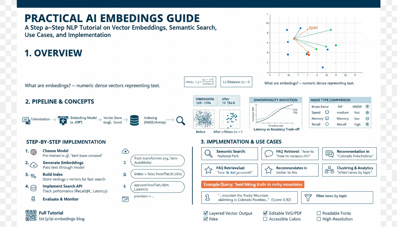
Embeddings turn text into numeric vectors so machines can reason about meaning: similar phrases map to nearby points in high‑dimensional space. Distance (commonly cosine similarity) reflects semantic relatedness rather than literal token overlap, which lets you match paraphrases, cluster topics, and rank search results. Think of an embedding as a compact fingerprint capturing context: words like “bank” will have different embeddings depending on surrounding text, while sentence or document embeddings compress that context into one vector.
Simple arithmetic on vectors reveals semantic structure (e.g., vector(“king”) − vector(“man”) + vector(“woman”) lands near vector(“queen”)), illustrating how relationships are encoded directionally. Practically, choose embedding dimension and model by task: higher dimensions often capture subtler distinctions but cost more in storage and nearest‑neighbor search. Normalize vectors when using cosine similarity, use approximate nearest neighbor (ANN) indexes for speed at scale, and chunk long documents with overlap then aggregate or store per‑chunk embeddings for retrieval.
Beware pitfalls: out‑of‑domain text can produce poor semantics; averages of token vectors may lose order and nuance; and small cosine differences can be meaningful or noisy depending on the model. Quick heuristics: use prebuilt sentence/document embeddings for semantic search, fine‑tune or adapt models for domain specificity, and validate similarity thresholds on held‑out examples. Visualize low‑dim projections (PCA/UMAP) to sanity‑check clusters before productionizing.
Choosing embedding models
Start by matching model capability to the task and constraints: semantic search and retrieval benefit from pretrained sentence/document encoders; clustering and topic discovery prefer higher‑capacity vectors; classification or embedding-based features may work with smaller, faster models. Always weigh accuracy against latency, cost, and storage: larger models usually yield finer semantic distinctions but increase inference time and vector size.
Consider domain fit and multilingual needs. If your text is specialized (legal, medical, code), a general-purpose model may miss nuances—either fine‑tune, use domain‑adapted models, or add domain-specific vocabulary. For multilingual applications choose models trained on the target languages. Account for privacy and deployment: on‑device/local models reduce data exposure; hosted APIs simplify maintenance but add cost and potential compliance constraints.
Evaluate choices with a compact benchmark: create positive/negative pairs or a held‑out retrieval set, then measure recall@k, MRR, and the cosine‑similarity gap between positives and hard negatives. Run latency, throughput, and cost tests at expected scale. Use these results to pick dimension size and whether to compress or reduce dimensions for production.
Operational tips: normalize vectors for cosine searches, chunk long documents with meaningful overlap, persist embeddings for identical inputs to avoid recomputation, and match your ANN index to vector dimensionality. Monitor embedding drift as data evolves and plan for periodic re‑embedding or lightweight fine‑tuning. A practical heuristic: start with a well‑tested sentence encoder, benchmark on your data, then trade up or adapt only when necessary.
Preparing and cleaning text
Clean, consistent text is the foundation for useful embeddings: your goal is to preserve semantic content while removing noise that confuses models or inflates your index.
Start by normalizing character encoding (Unicode NFKC) and stripping control/zero‑width characters. Remove HTML, scripts, navigation, and boilerplate (headers, footers, ads) so only meaningful content remains. Collapse excessive whitespace and normalize newlines to single spaces for sentence-based chunking while keeping sentence delimiters for later splitting.
Preserve semantic tokens: avoid aggressive stop‑word removal or heavy stemming because embeddings rely on context. Prefer light normalization—lowercase if your model is case‑insensitive; otherwise keep case. Expand or normalize contractions when they improve clarity for your domain. Replace or mask sensitive or noisy tokens—map URLs, emails, phone numbers, and long UUIDs to placeholders (e.g., https://example.com →
Handle special domains intentionally: keep code formatting and inline punctuation for code/documentation; detect language and route non‑target languages to multilingual models or translate before embedding. For long documents, split on sentence boundaries into overlapping chunks (e.g., 200–500 tokens with 20–50% overlap) to preserve context for retrieval.
Finish with deduplication, consistent tokenization, and a small human or automated QA pass to validate that preprocessing preserved meaning. A minimal pipeline: normalize → strip HTML/boilerplate → mask PII/URLs → sentence split → chunk with overlap → dedupe → tokenize for the embedding model.
Generating embeddings with Python
Use a pretrained sentence encoder for the simplest, most reliable embeddings or run a transformer and apply pooled aggregation yourself. The example below uses sentence-transformers for one-line encoding, then shows a raw-transformer mean-pooling pattern so you understand what’s happening under the hood.
# sentence-transformers (recommended)
from sentence_transformers import SentenceTransformer
import numpy as np
model = SentenceTransformer('all-MiniLM-L6-v2')
texts = ['Search query', 'Document text...']
embs = model.encode(texts, batch_size=64, show_progress_bar=True, convert_to_numpy=True)
# L2-normalize for cosine similarity
embs = embs / np.linalg.norm(embs, axis=1, keepdims=True)

# persist
np.save('embeddings.npy', embs)
# raw transformers + mean pooling (when you need control)
from transformers import AutoTokenizer, AutoModel
import torch
tokenizer = AutoTokenizer.from_pretrained('all-MiniLM-L6-v2')
model = AutoModel.from_pretrained('all-MiniLM-L6-v2')
inputs = tokenizer(['some text'], return_tensors='pt', padding=True, truncation=True)
with torch.no_grad():
    out = model(**inputs)
last_hidden = out.last_hidden_state  # (batch, seq_len, dim)
mask = inputs['attention_mask'].unsqueeze(-1)
pooled = (last_hidden * mask).sum(1) / mask.sum(1)
pooled = torch.nn.functional.normalize(pooled, p=2, dim=1).cpu().numpy()
Process text in batches, keep the model loaded (reuse across calls), and compute on GPU for large workloads. For long documents, split into overlapping chunks (200–500 tokens, 20–30% overlap) and store per-chunk embeddings. Deduplicate identical inputs to avoid recomputation. Store embeddings plus metadata (doc id, chunk offset) and use an ANN index (FAISS/Annoy/Milvus) for fast nearest-neighbor retrieval. Always validate similarity thresholds and recall@k on a small held-out set before production.
Indexing vectors with FAISS
FAISS provides a production-ready way to store and query high‑dimensional embeddings with extremely fast nearest‑neighbor search. Choose an index that matches scale and update patterns: brute‑force IndexFlat for small datasets or exact recall, IVF (e.g., IndexIVFFlat) for large, memory‑efficient approximate search (requires training), and HNSW for fast, dynamic inserts without retraining. For cosine similarity, L2‑normalize vectors and use an inner‑product index (IndexFlatIP) so rankings match cosine scores.
Store a lightweight mapping from FAISS internal ids to your document metadata (doc id, chunk offset, text) using IndexIDMap or by keeping a separate key–value store. Always convert embeddings to float32 before adding and add in batches to avoid memory spikes. Persist indexes with faiss.write_index and reload with faiss.read_index for fast startup.
Example (Python):
import numpy as np
import faiss
vecs = np.asarray(embs, dtype='float32')
faiss.normalize_L2(vecs)            # for cosine
index = faiss.IndexFlatIP(vecs.shape[1])
index = faiss.IndexIDMap(index)     # keep external ids
ids = np.arange(len(vecs))
index.add_with_ids(vecs, ids)
# query
q = np.asarray([query_emb], dtype='float32')
faiss.normalize_L2(q)
D, I = index.search(q, k=10)
Tune IVF with nlist (number of coarse clusters) and nprobe (search breadth) to balance recall vs latency; larger nlist reduces memory per list but needs appropriate nprobe. Use HNSW parameters (M, efConstruction, efSearch) for faster recall at lower memory. For very large corpora consider FAISS GPU support, compressed indexes (PQ/OPQ) for storage savings, and periodic re‑indexing when embeddings change. Validate recall@k on held‑out queries and keep metadata separate for flexible retrieval and filtering.
Evaluating and optimizing search
Start by defining clear success metrics: recall@k and MRR capture relevance for retrieval, precision@k helps when top results must be accurate, and latency/throughput measure user experience. Build a small held‑out evaluation set with labeled positives and hard negatives drawn from real queries; include edge cases and ambiguous queries to surface failure modes. Measure the cosine gap between positives and hard negatives and use ROC or precision‑recall curves to pick operating points rather than a single arbitrary threshold.
Optimize the stack iteratively. First, tune embedding and preprocessing: normalize vectors for cosine, experiment with chunk sizes/overlap, and test domain‑adapted models or lightweight fine‑tuning using collected hard negatives. Next, tune the ANN index: for IVF adjust nlist and nprobe to balance recall vs latency; for HNSW tune M and efSearch; for production, measure recall@k as you change these parameters rather than relying on synthetic benchmarks. When compressing vectors (PQ/OPQ), validate loss in recall at target k and consider hybrid indexes that keep a small exact store for top candidates.
Improve ranking with a two‑stage approach: retrieve a moderately large candidate set (e.g., 100) with ANN, then rerank with a cross‑encoder or a learned reranker to boost precision. Combine semantic scores with lexical signals (BM25) for hard keyword matches and apply lightweight score calibration so scores are comparable across queries. Log entire user interactions and store feedback as training signals; re‑evaluate thresholds and models periodically to catch drift. Use A/B tests and human assessment on sampled queries to confirm metric gains translate to user value.
Automate evaluation pipelines, include latency and cost in tradeoff decisions, and schedule incremental re‑embedding when data or behavior shifts to keep search quality stable.