Common SQL Patterns Overview
Building on this foundation, the practical toolbox you reach for day-to-day is a small set of proven SQL patterns that solve recurring problems. Right away, prioritize learning canonical SQL patterns and SQL query patterns that handle filtering, joining, aggregation, and row-level transformations — these recur across analytics, ETL, and OLTP workloads. We’ll treat each pattern as a tradeoff: when you prefer clarity, when you need raw performance, and when maintainability wins out. This front-loaded view helps you recognize opportunities to replace ad-hoc queries with repeatable, testable patterns.
Start with the basics: selection, predicates, and joins. Selection and predicate patterns (project only needed columns, push selective predicates early) reduce I/O and memory pressure. Join patterns — inner, left, semi, anti, and cross — express intent: use semi-joins to test existence, anti-joins to exclude, and left joins when you need outer-presence semantics. How do you choose between a NOT EXISTS anti-join and an anti-left-join-where-null? Use NOT EXISTS for clarity and predictable performance on indexed keys; prefer left-join-where-null only when the planner on your RDBMS has known deficiencies.
Aggregation and grouping patterns are where business metrics live. Use GROUP BY for rollups and HAVING to filter aggregated results, and prefer window functions when you need aggregates alongside row-level detail. For multi-level aggregation (daily, weekly, total) use GROUPING SETS or WINDOW framing to avoid multiple scans. For example, computing per-user latest and total spend in one pass: a window for latest timestamp and a GROUP BY for totals gives both granular and summary views without duplicating reads.
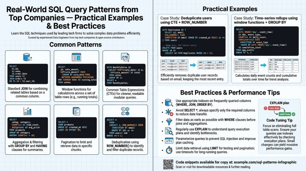
Deduplication and Top-N patterns are best solved with window functions. When you want the latest record per key or the top K items per partition, use ROW_NUMBER() or RANK() with PARTITION and ORDER clauses rather than expensive correlated subqueries. Example:
WITH ranked AS (
  SELECT *, ROW_NUMBER() OVER (PARTITION BY user_id ORDER BY updated_at DESC) AS rn
  FROM events
)
SELECT * FROM ranked WHERE rn = 1;
This pattern is deterministic, index-friendly (when you have an index on user_id, updated_at), and much easier to maintain than nested subselects.
Common structuring patterns include Common Table Expressions (CTEs) and modularized subqueries. Use CTEs to break a complex transformation into named steps; they act like readable pipeline stages. Recursive CTEs are the canonical option for hierarchical traversals (organization charts, bill-of-materials), while non-recursive CTEs make debugging and testing easier by letting you SELECT from intermediate results. Keep an eye on materialization behavior in your engine — some CTEs are inlined, others are materialized, and that choice impacts memory and execution plans.
Operational patterns — upserts, pagination, and anti-pattern avoidance — are where production systems fail if ignored. Use MERGE or INSERT … ON CONFLICT for idempotent upserts in OLTP; prefer key-based upserts to avoid race conditions. For pagination, prefer keyset (seek) pagination over OFFSET for large offsets to keep latency stable. Finally, watch for common anti-patterns: SELECT *, excessive cross joins, and repeated full-table scans. These patterns and their tradeoffs guide the queries we write and optimize; in the next section we’ll apply them to concrete examples drawn from production-grade analytics and service workloads to show how they behave under real data distributions.
Sargable Queries and Indexing
Building on this foundation, the simplest way to win consistent query performance is to write sargable queries and understand how indexing interacts with predicates. Sargable (search-argument-able) predicates let the database use an index seek instead of a full scan; that difference often turns a query from minutes to milliseconds on large tables. In this section we’ll show concrete rewrites, explain how composite and covering indexes change planner behavior, and give practical rules you can apply immediately to OLTP and analytics workloads.
The core idea is straightforward: the query optimizer can only use an index when the predicate lets it match values directly. If you wrap a column in a function, apply arithmetic to it, or use a leading wildcard in a LIKE, you typically prevent index seeks and force a scan. That behavior increases I/O and CPU, and it blows up as table size grows. For predictable, repeatable performance you must treat predicate shape as part of your schema design and indexing strategy.
Here are common non-sargable-to-sargable rewrites you can apply today. If you write WHERE DATE(created_at) = ‘2025-01-01’ the engine must compute DATE(created_at) for every row; rewrite it to a half-open range so the index on created_at can be used:
-- non-sargable
SELECT * FROM events WHERE DATE(created_at) = '2025-01-01';

-- sargable
SELECT * FROM events
WHERE created_at >= '2025-01-01' AND created_at < '2025-01-02';
Similarly, avoid expressions on the indexed column: WHERE quantity * 1.0 > 10 should become WHERE quantity > 10 (or index an expression if your RDBMS supports it). For text matching, WHERE name LIKE '%smith' defeats the index; WHERE name LIKE 'smith%' remains sargable. When you have multiple ORs across different indexed columns, consider rewriting with UNION ALL or use IN on a single column to preserve index usage.
Composite indexes and covering indexes change how you structure predicates and projections. If you frequently filter by user_id and then need the latest updated_at, an index on (user_id, updated_at DESC) lets the planner satisfy both the filter and the ordering with a single index seek and a limit. A covering index that includes the columns you SELECT (for instance, INCLUDE (status, amount) in SQL Server or CREATE INDEX ... (a,b) INCLUDE (c)) can avoid touching the base table entirely, producing an index-only scan. We used this pattern earlier with ROW_NUMBER() to make Top-N per-user queries deterministic and index-friendly: the index orders match the partitioning and ordering of the window function.
When simple rewrites aren’t feasible, use advanced indexing: functional (expression) indexes and partial (filtered) indexes let you keep predicates sargable without changing application logic. For example, if you must query lower(email), create an index on lower(email) instead of applying the function at runtime. Partial indexes reduce maintenance cost by indexing only rows that matter (e.g., WHERE is_active = true) which is useful when a small subset of rows receives most queries. Remember these indexes add write overhead and storage; measure the tradeoff before blanket application.
In practice we rely on EXPLAIN and cardinality statistics to validate assumptions. Run EXPLAIN ANALYZE on suspect queries, confirm whether the planner chooses an index seek or a scan, and iterate: sometimes adding a small covering index removes a costly sort or large random I/O. Ask yourself: When should you accept a table scan? Accept scans for ad-hoc, low-frequency analytical queries or when the table is small relative to the cost of maintaining complex indexes; otherwise, invest in sargable rewrites or targeted indexes. With that mindset—shape predicates to match indexes, use composite/covering or functional indexes where appropriate, and validate with the planner—you’ll convert many slow queries into reliable, production-grade patterns that scale.
Joins and Aggregation Techniques
Joins and aggregation are where business metrics meet data movement — get them wrong and queries either produce incorrect results or consume massive resources. In the next few paragraphs we’ll show practical, production-ready SQL patterns that reduce shuffle, exploit indexes, and keep aggregation work proportional to the data you actually need. How do you decide whether to join then aggregate or aggregate then join? The answer drives both performance and correctness for common analytics and ETL workloads.
Start by pre-aggregating wide, high-cardinality tables before joining whenever possible. If you have a large events table and need daily counts per user joined to a relatively small user dimension, aggregate the events first and then join the small dimension: this reduces rows moving through the join and makes the join algorithm cheaper. Example pattern:
WITH daily AS (
  SELECT user_id, event_date, COUNT(*) AS events
  FROM events
  WHERE event_date BETWEEN '2025-01-01' AND '2025-01-31'
  GROUP BY user_id, event_date
)
SELECT u.user_id, u.country, d.event_date, d.events
FROM daily d
JOIN users u USING (user_id);
This approach trades compute for network and memory savings and is especially effective when your aggregation keys are a strict subset of the join keys. When you can push aggregation into the source (pushdown) or into a materialized aggregate table, you consistently reduce query latency.
Understand how join algorithms and indexing affect aggregation strategies. Merge joins thrive when both sides are pre-sorted (or when there’s an index that matches the join ordering), while hash joins are good for large unsorted builds but require memory proportional to the build side. If the planner can use an index to satisfy ordering and filtering, you often avoid a separate sort step; design composite indexes that match your most common join+grouping patterns (for example, (user_id, event_date DESC)). We prefer to force the planner into an index-friendly path by aligning partitioning, ordering, and index keys rather than relying on in-memory sorts for large datasets.
Semi and anti patterns express intent more clearly than boolean join hacks; use them to avoid unnecessary aggregation after filtering. Prefer NOT EXISTS or EXISTS for anti/semi logic because they avoid building a full join intermediate and are typically index-friendly:
-- exclude users who have a canceled flag in recent_orders
SELECT u.user_id
FROM users u
WHERE NOT EXISTS (
  SELECT 1 FROM recent_orders r WHERE r.user_id = u.user_id AND r.status = 'canceled'
);
Use LEFT JOIN … WHERE right.id IS NULL only when you’ve validated planner behavior on your engine, otherwise NOT EXISTS provides clearer semantics and predictable performance.
When you need multiple rollups in a single scan, use GROUPING SETS, CUBE, or the FILTER clause to avoid repeated scans. GROUPING SETS lets you compute per-user, per-day, and grand totals in one pass, which is cheaper than three separate GROUP BY queries. Example:
SELECT
  COALESCE(user_id, 'ALL') AS user_id,
  event_date,
  SUM(amount) AS total_amount
FROM events
WHERE event_date >= '2025-01-01'
GROUP BY GROUPING SETS ((user_id, event_date), (user_id), ());
Combine aggregates with window functions when you need both row-level detail and summary metrics without extra joins. For example, compute each transaction’s rank within a user partition and the user’s 30-day rolling sum using ROW_NUMBER() and SUM() OVER (PARTITION … RANGE) in the same query to avoid separate aggregation steps.
Operationalize aggregation by thinking about incremental maintenance and memory limits. Materialized views or incremental aggregate tables remove repeated heavy scans; approximate aggregation (e.g., HyperLogLog for distinct counts) can give huge wins when exactness isn’t required. Always validate with EXPLAIN ANALYZE and cardinality stats: measure whether a pre-aggregation reduced rows, whether the planner used an index, and whether a hash build spilled to disk. With those checks in place we’ll keep joins and aggregation both correct and performant as data grows.
Window Functions for Analytics
Building on the previous patterns, window functions are the natural next tool when you need row-level context alongside aggregates in analytics queries. Window functions let you compute running totals, moving averages, ranks, and top-N results without collapsing rows into summaries, which means you can keep transactional detail and summary metrics in the same pass. In analytics workloads where scan cost matters, combining window functions with selective predicates and proper indexing often reduces overall work compared with multiple GROUP BY passes. How do you pick the right window framing or aggregate for a production pipeline?
Start by thinking in three parts: partitioning, ordering, and framing. Partitioning with PARTITION BY scopes the calculation (for example, per user, per session), ordering establishes temporal or score order, and the frame (ROWS or RANGE) defines which rows contribute to each output row. Use partitioning to limit memory pressure and to make parallelism explicit to the planner; for instance, partition by user_id and country only when your business logic requires that two-dimensional scope. This mental model keeps window functions predictable and aligns them with the indexing and join strategies discussed earlier.
Framing is where queries diverge in intent and performance. ROWS frames are row-count based and deterministic across storage layouts, so prefer ROWS BETWEEN n PRECEDING AND CURRENT ROW when you need exactly N prior rows (for example, a 30-transaction moving average). RANGE frames are value-based and let you express time windows like “last 30 days” if your engine supports value-based intervals, which is more intuitive for time-series analytics but can be planner-dependent. When should you prefer ROWS framing over RANGE framing? Choose ROWS for fixed-size windows and RANGE for value/time-based windows when consistent behavior across ties and nulls matches your requirements.
Practical patterns matter in production. For deduplication and stable Top-N results you’ll combine ROW_NUMBER() with a deterministic ORDER BY that includes tie-breakers (unique surrogate key or timestamp). For sessionization, use LAG() and LEAD() to detect boundaries and then SUM() as a windowed flag to assign session ids in one scan. For churn and cohort analytics, compute per-user retention curves using COUNT(*) OVER (PARTITION BY cohort_id ORDER BY week RANGE BETWEEN INTERVAL '0' DAY AND INTERVAL '28' DAY) (or the dialect-appropriate equivalent) to avoid separate JOINs between cohorts and events.
Here are two compact, engine-agnostic examples to illustrate the approach. For a 30-transaction moving sum per user you can use:
SELECT *,
  SUM(amount) OVER (PARTITION BY user_id ORDER BY created_at ROWS BETWEEN 29 PRECEDING AND CURRENT ROW) AS moving_30_rows
FROM transactions
WHERE created_at >= '2025-01-01';
For a 30-day rolling sum (if your SQL dialect supports interval-based RANGE frames):
SELECT *,
  SUM(amount) OVER (PARTITION BY user_id ORDER BY created_at RANGE BETWEEN INTERVAL '29 days' PRECEDING AND CURRENT ROW) AS moving_30_days
FROM transactions
WHERE created_at >= '2025-01-01';
Always validate with EXPLAIN and measurements. Window functions can increase memory usage because the engine may need to buffer partition frames; mitigate this by filtering early, partitioning on higher-cardinality keys only when needed, and creating composite indexes that match PARTITION BY + ORDER BY to allow index-ordered scans. When a partition is extremely large, consider pre-aggregating or bucketing time ranges and then applying windows on the reduced set to avoid spills.
Finally, think about maintainability and testability: encapsulate complex window logic in a named CTE so you can unit-test intermediate results and reason about edge cases like ties and null timestamps. In analytics pipelines where correctness matters, include explicit tie-breakers in ORDER BY, document the choice of ROWS vs RANGE, and add regression tests for boundaries (first/last rows, partition edge cases). Taking this approach makes window functions a predictable, high-impact part of your SQL toolbox for analytics.
Partitioning, Sharding, and Materialized Views
Partitioning, sharding, and materialized views are the three pragmatic levers we reach for when a single-table scan or a monolithic index can no longer meet latency or scale targets. In practice you’ll use partitioning to prune I/O on large tables, sharding to distribute write and storage load across nodes, and materialized views to avoid repeated heavy aggregation work; each comes with tradeoffs in complexity, maintenance, and freshness. When should you choose partitioning over sharding, or when are precomputed aggregates via materialized views the right approach? We’ll walk through decision criteria and concrete patterns you can apply today.
Start with partitioning when your workload has a natural, stable dimension you can prune on—time, geo, or tenant id. Partitioning at the database level (for example RANGE partitioning on created_at or LIST partitioning on region) lets the planner skip irrelevant partitions, reducing scan and I/O cost while keeping transactional semantics intact. Take this PostgreSQL-style example:
CREATE TABLE events (
  id bigint PRIMARY KEY,
  user_id bigint,
  created_at timestamptz,
  payload jsonb
) PARTITION BY RANGE (created_at);
-- then create monthly partitions
CREATE TABLE events_2026_01 PARTITION OF events FOR VALUES FROM ('2026-01-01') TO ('2026-02-01');
Partition pruning works best when you write sargable predicates against the partition key (as we discussed earlier), so push date or tenant filters into WHERE clauses and create supporting indexes on (partition_key, ordering_column) to allow index-only scans. Partitioning keeps the operational complexity low because backups, restores, and VACUUM/maintenance can be targeted per partition; however, it doesn’t solve single-node capacity limits—if a single partition becomes too large you’ll hit the same scaling wall.
Sharding is the step you take when you must scale storage and writes horizontally across multiple database instances. Choose a shard key with stable cardinality and an access pattern that keeps hot-spotting rare—user_id modulo N is common, but consistent hashing or directory-based routing gives more flexible rebalancing. Sharding changes how you think about joins and transactions: cross-shard joins force fan-out or require denormalization, and distributed transactions add latency and operational risk. For example, instead of a global join between orders and payments, you often denormalize the payment status into the orders shard or maintain a lightweight lookup service to route reads to the correct shard.
Materialized views are our tool for expensive, repeatable aggregations that you don’t want to compute on every request. Create a materialized view when a query is run frequently, the underlying data changes at controlled velocity, and slightly stale results are acceptable or can be updated incrementally. Example pattern in PostgreSQL:
CREATE MATERIALIZED VIEW mv_daily_user AS
SELECT user_id, date_trunc('day', created_at) AS day, COUNT(*) AS cnt
FROM events
GROUP BY user_id, date_trunc('day', created_at);
-- refresh strategy
REFRESH MATERIALIZED VIEW CONCURRENTLY mv_daily_user;
Decide on refresh semantics: REFRESH ON COMMIT gives strong freshness but high write cost; scheduled or incremental refreshes (where supported) balance latency and throughput. Also ensure the materialized view is indexed to support common query predicates—an index on (user_id, day) often turns the view into an index-backed lookup that replaces heavy GROUP BY scans. Remember that materialized views add write overhead and storage, so measure write amplification and validate that query rewrite by the planner is actually using the view.
Combine these patterns rather than view them as exclusive choices. For example, partition your events table by month, shard tenants across nodes, and maintain a per-shard materialized view for the heavy monthly aggregates; this reduces cross-shard traffic and makes refresh operations local and parallelizable. Test the operational flows: how you reshard, how you refresh views after backfills, and how you rebuild a partition without downtime. We recommend automated scripts for partition creation, consistent-hash ring management for shards, and idempotent refresh jobs for materialized views so you can recover and scale predictably.
Taking these ideas further, instrument and validate with explain plans, metrics, and replayed production workloads before committing to a design. As we discussed earlier with sargable predicates and composite indexes, the right index choices and predicate shapes determine whether partition pruning and materialized-view lookups actually avoid full scans. Next, we’ll apply these combined strategies to concrete production-grade queries to show how they behave under skewed distributions and bursty traffic.
EXPLAIN, Profiling, and Tuning
Building on this foundation, the fastest-looking query can still be a production liability if you don’t inspect its execution plan and profile actual resource use. Start with EXPLAIN to see the planner’s chosen execution plan and then run EXPLAIN ANALYZE to observe real execution behavior — estimated rows versus actual rows, chosen join algorithms, and whether the planner predicted costs accurately. How do you know which part of the query is the real bottleneck? The difference between estimated and actual cardinality is often the single best clue that you must do deeper query profiling and query tuning.
When you run EXPLAIN ANALYZE, read it like a performance hypothesis: the top-level node shows total time, child nodes show per-step costs, and the estimated vs. actual rows column reveals cardinality problems. If an index seek was expected but a sequential scan occurred, look at predicate sargability and whether statistics or parameterization forced a scan. Also enable buffer and timing reporting (for engines that support it) to learn whether time was spent CPU-bound, waiting on I/O, or performing heavy sorts and temporary file spills; those metrics guide whether to add an index, increase work_mem, or rewrite the query.
Profiling goes beyond the plan text: capture system-level waits, temporary file usage, and per-query resource counters so you can attribute latency to I/O, CPU, or memory pressure. Use engine-native extensions or performance views to aggregate hot SQL (for example, statement-level stats), and reproduce a slow query with representative constants under EXPLAIN ANALYZE instead of synthetic minidata. In production-like replays you’ll see plan instability (plans that perform well on small samples but fail at scale), and profiling data helps decide whether to change schema, add a covering index, or pre-aggregate results into a materialized view.
Cardinality and statistics drive most bad plans. If the planner’s estimates are off, it will choose suboptimal join orders or join types; stale or low-resolution histograms are typical culprits for skewed distributions. Increase sampling (statistics_target), collect multi-column or extended statistics for correlated predicates, and consider partial or functional indexes when only a subset of values is hot. In many real-world cases a single highly-skewed column (for example, 95% of rows share the same status) explains why an index isn’t used and why a hash join spills to disk.
Parameter-sensitive plans and plan caching are another practical pitfall. Prepared or parameterized statements may be compiled using an unlucky bind value, producing a cached plan that underperforms for other inputs. When you suspect this, compare plans for literal-bound queries versus prepared statements, test with representative bind values, and, if necessary, use planner hints, recompile strategies, or adaptive execution features your engine offers. Balance these fixes against overhead: forcing recompiles reduces caching benefits, while per-value plans increase compilation pressure.
A pragmatic tuning workflow accelerates decisions: identify high-cost queries by frequency × latency, reproduce with production-like data, run EXPLAIN ANALYZE and collect profiler metrics, then iterate — rewrite predicates for sargability, add composite or covering indexes that align with partitioning and ORDER BY, and, if needed, introduce pre-aggregates or partition pruning. Measure the change in scanned rows, buffer hits, and wall-clock time; a tenfold drop in scanned rows is usually more valuable than micro-optimizing a CPU-bound expression.
As we move to concrete production examples, keep one rule: validate every change with explain plans and regression tests against representative datasets. Store baseline plans, watch for drift after stats updates or schema changes, and automate alerts for plan regressions so query tuning becomes a repeatable engineering practice rather than ad-hoc firefighting. This disciplined approach converts EXPLAIN, profiling, and tuning from occasional troubleshooting tools into part of your continuous performance toolkit.