Problem Overview and Goals
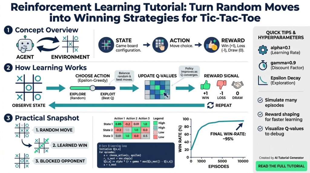
Reinforcement learning and Tic-Tac-Toe are a compact laboratory for turning random moves into winning strategies, and that’s exactly why this project matters. How do you turn random moves into a reliable, winning strategy using reinforcement learning? We’ll treat the game as a sequential decision problem: the agent observes the board, selects an action, receives a reward, and updates its policy. This section frames the practical problems we solve, the measurable goals we set, and the constraints that drive design trade-offs.
The core problem is a combination of sparse rewards, exploration-exploitation trade-offs, and representational choices. You’ll face sparse terminal rewards because most feedback arrives only when the game ends (win/draw/loss), so naive updates are slow to assign credit to individual moves. The action space is small but discrete, and the environment is deterministic with perfect information, which simplifies modeling but raises an expectation: we should be able to converge to optimal play if learning and exploration are handled correctly. Therefore we must design training that balances exploration of random moves with systematic policy improvement.
Our goals translate abstract learning objectives into concrete success criteria you can measure during development. First, we want an agent that consistently beats a baseline random player with a high win rate (target 90%+ over 1,000 games). Second, we aim for sample-efficient learning: minimize episodes-to-competence so experiments iterate quickly. Third, we want a policy that generalizes across board symmetries (rotations/reflections) rather than memorizing states. Finally, we treat achieving optimal or draw-level play against a perfect opponent as a stretch goal—this demonstrates provably sound learning and robust winning strategies.
Constraints and assumptions will govern algorithm choice and implementation details. We assume the environment is fully observable and deterministic, so model-based approaches (table-driven Q-learning or small neural nets) are viable. Compute and memory budgets are modest because Tic-Tac-Toe has at most 3^9 possible board encodings when including empty spaces; that allows tabular methods or compact function approximators. Episodes are short (max 9 moves), so training loops must handle many episodes efficiently and exploit symmetry to reduce state space. Finally, we’ll assume reproducible, seeded randomness so you can debug exploration behavior reliably.
To evaluate progress and drive learning, choose measurable metrics and clear training signals. Track win/draw/loss rates against fixed opponents and plot moving averages to spot plateaus. Use an epsilon-greedy exploration schedule so the agent explores early and exploits later; for example:
# epsilon-greedy policy (pseudocode)
def select_action(state, Q, epsilon):
    if random() < epsilon:
        return random_valid_action(state)
    return argmax_action(Q[state])

# simple Q update
Q[s,a] += alpha * (reward + gamma * max_a' Q[s',a'] - Q[s,a])
These snippets show how we turn episodic rewards into incremental value updates that reinforce winning moves. Reward shaping (small negative step penalty or positive reward for capturing two-in-a-row) can speed convergence, but we’ll use it sparingly to avoid altering optimal strategies.
With the problem framed and the goals defined, we can pick algorithms and implementation patterns that match constraints and metrics. Next we’ll examine algorithm choices—tabular Q-learning, SARSA, and policy-gradient methods—deciding when each fits the requirement for sample efficiency, interpretability, and convergence to winning strategies. By keeping goals measurable and constraints explicit, you’ll be able to iterate quickly and diagnose why learning stalls or why random moves persist in the policy.
Representing Game State
Building on this foundation, the way you encode the game state dramatically affects sample efficiency, generalization, and whether tabular or function-approximation methods make sense. Representing the game state for a Tic-Tac-Toe reinforcement learning agent isn’t just bookkeeping: it’s the interface between environment dynamics and your learning algorithm. How do you choose an efficient state representation for Tic-Tac-Toe that makes learning fast and robust? We’ll show compact, canonical, and neural-friendly encodings and explain when to pick each one so you can stop wasting episodes on redundant states.
A compact, lossless option is a base-3 (ternary) encoding: map empty=0, X=1, O=2 and interpret the 9 cells as digits in a base-3 integer to produce a unique state index in [0, 3^9). This integer representation is perfect for tabular Q-learning because it gives O(1) indexing into arrays or dictionaries and minimizes memory overhead. For example, in Python you can convert a board list to an index with:
index = sum(cell * (3**i) for i,cell in enumerate(board))
Use that index as a Q-table key or as the state hash when persisting experience.
Because the environment has symmetries, canonicalization is the next lever to shrink the effective state space. Map each observed board to its canonical form by applying all 8 rotations/reflections and picking the lexicographically smallest (or largest) encoding; this reduces equivalent states and forces the agent to learn symmetric strategies once rather than eight times. For tabular methods this yields big wins in sample efficiency; for function approximators you can either train on canonical states or augment your training batch with symmetric variants to encourage invariance. Keep in mind canonicalization requires you to also transform actions back to the original orientation when selecting moves in the environment.
Action representation and legality constraints should be explicit in your state-action interface. Represent actions as integers 0–8 (cell indices) and always provide a legal-move mask derived from the current board so the policy can ignore illegal outputs during argmax or softmax sampling. In practice, implement action masking inside your selection routine: set Q[state, illegal_action] = -inf (or mask logits before softmax) to prevent illegal choices. This makes policy evaluation deterministic and prevents wasted updates on impossible moves, which is especially useful given sparse terminal rewards.
If you move to neural networks, prefer structured feature tensors over flat integers for better generalization. A common pattern is a 3x3x3 tensor with three channels: X-occupancy, O-occupancy, and empty (or add a fourth channel indicating current player to move). Convolutional architectures on that tensor easily learn spatial patterns like two-in-a-row, while an MLP on a flat one-hot vector works but generalizes less well across rotations. Also consider adding a parity scalar (turn count mod 2) as an extra input channel to disambiguate identical board layouts with different players to move; this small feature prevents the agent from conflating states that require different optimal actions.
Representation choices drive downstream engineering trade-offs, so make them deliberate. If you want interpretability and provable convergence, use the base-3 index plus canonicalization and tabular Q; if you want smoother generalization across noisy opponents, use convolutional inputs with symmetry augmentation. Remember to persist state hashes or tensor checkpoints so you can resume training and reproduce experiments. Taking these representational steps will shrink the effective state space, speed convergence in reinforcement learning, and make your agent’s policy easier to debug as you progress to algorithm selection and reward-shaping.
Designing Rewards and Episodes
Building on this foundation, getting rewards and episodes right is the single most important lever you can pull to turn random moves into robust play in reinforcement learning. Early feedback should tell you something useful about move quality without changing the optimal strategy, and episode boundaries must reflect the game dynamics so learning signals remain meaningful. If you design rewards poorly you’ll see fast-but-brittle policies or slow learning from sparse terminal outcomes, so we’ll focus on practical patterns that speed credit assignment while preserving optimal play.
The fundamental trade-off is between sparse terminal rewards and informative, shaped rewards that guide learning. Sparse rewards (win=+1, draw=0, loss=-1) are correct but make credit assignment hard because most updates occur only at episode end. How do you assign credit to early moves? Potential-based reward shaping is a principled answer: add a shaping term F(s,a,s’) = gamma * Phi(s’) – Phi(s) where Phi is a potential function over states. This preserves policy invariance while providing dense gradients toward useful subgoals, so you can accelerate learning without changing the optimal policy.
For Tic-Tac-Toe concrete choices work well. Use terminal rewards of +1 (win), 0 (draw), -1 (loss) and add a small step penalty like -0.01 per move to discourage gratuitous delays and encourage finishing lines. Define Phi(s) as a count of “two-in-a-row” opportunities for the learning agent minus the opponent’s opportunities; that makes F positive when we increase imminent win chances and negative when we open the opponent. Keep shaping magnitudes small (e.g., Phi scaled to 0.0–0.5) so the agent still prioritizes the terminal +1 reward over greedy shaping exploits.
Episode structure should mirror gameplay and training objectives. Treat a full board or any terminal win/loss as an episode end and cap episodes at nine moves, but allow early termination on a detected win to save compute. Start training against a random opponent for broad coverage, then use a curriculum or opponent schedule: gradually introduce stronger heuristics, self-play, or a minimax agent. Evaluate in dedicated evaluation episodes (no exploration) — for example, run 1,000 evaluation games every 5000 training episodes — so you separate noisy online learning from true policy performance.
Adopt training patterns that reinforce credit assignment across episodes. For tabular Q-learning, update Q-values stepwise with TD targets every move and optionally apply Monte Carlo returns at episode end to stabilize long-horizon credit. If you use function approximation, normalize and clip shaped rewards to prevent gradient explosions and prefer TD(lambda) or eligibility traces to propagate terminal signals faster across preceding states. Instrument per-episode diagnostics: moving averages of win/draw/loss, average episode length, and frequency of shaped-event triggers (two-in-a-row created/blocked) so you can diagnose whether shaping accelerates the right behaviors.
Finally, connect reward and episode choices to the representations and algorithms we discussed earlier. Because you canonicalize symmetric boards and mask illegal actions, shaped rewards translate to fewer distinct signals and thus faster generalization across rotated states. Measure progress with clear metrics and use shaping only as a training scaffold — once the agent reliably exceeds your baseline (for example, 90%+ wins vs random over 1,000 games) reduce shaping to zero and verify the policy still performs. With careful shaping, explicit episode boundaries, and a progressive opponent schedule, you’ll convert sparse feedback into actionable learning and be ready to choose the algorithm (tabular Q, SARSA, or policy gradients) that best fits your performance and interpretability goals.
Select Q-learning or SARSA
Choosing between Q-learning and SARSA is one of the first practical decisions you make when turning Tic-Tac-Toe randomness into a reliable policy using reinforcement learning. Both algorithms are lightweight tabular temporal-difference methods that fit the small, deterministic state space we’ve canonicalized earlier, but they differ in how they bootstrap future value and how that interacts with exploration. Front-load this decision: do you want an algorithm that learns the greedy optimal value regardless of how you explore, or one that learns the value of the actual exploration policy you run during training? Your choice shapes stability, sample efficiency, and how you interpret early training behavior.
The core technical difference is on-policy versus off-policy bootstrapping. SARSA (State-Action-Reward-State-Action) updates Q(s,a) toward the return following the action actually taken in the next state, so it learns the value of the epsilon-greedy policy you execute; Q-learning updates Q(s,a) toward the maximum next-state value, effectively estimating the value of the greedy policy regardless of exploratory actions. In practice this means Q-learning uses optimistic bootstrapping (max over next actions) while SARSA uses the agent’s sampled next action to form the TD target. Because we mask illegal moves and canonicalize states, both algorithms get cleaner signals, but their update targets still encode different assumptions about future behavior.
Exploration behavior makes these differences concrete in gameplay. SARSA tends to produce safer policies during training because it internalizes the risk introduced by epsilon exploration: if an exploratory move can be punished by the opponent, SARSA will lower the value of moves that lead into risky states under the current exploration rate. Q-learning can be more aggressive: it may raise values for moves that look good under greedy play even if exploratory steps often lead to bad outcomes. For example, allowing the opponent a two-in-a-row by exploring a “promising” diagonal might be penalized sooner under SARSA, whereas Q-learning might propagate optimism and take longer to correct unless exploration decays.
From a convergence and sample-efficiency perspective, both algorithms are well-suited to Tic-Tac-Toe’s tabular setting and will converge under standard assumptions (sufficient exploration, decaying alpha, etc.). However, SARSA often shows smoother learning curves when you evaluate the policy you actually run during training, while Q-learning can reach a stronger final greedy policy slightly faster once exploration is reduced. Because we already reduce the effective state space with symmetry canonicalization and mask illegal actions, expect both methods to require relatively few episodes to surpass a random baseline — but monitor moving averages to detect optimistic plateaus with Q-learning.
Practically, pick Q-learning when your workflow separates training and evaluation: train with exploration, then switch to a greedy policy for evaluation or deployment and you want the algorithm to target that greedy behavior directly. Pick SARSA when you need stable, predictable behavior during interactive training (for debugging, curriculum learning, or when opponents are stochastic). Tune similarly for both: alpha in 0.1–0.3 is a good starting point for tabular updates, gamma near 0.99 preserves long-term rewards, and an epsilon schedule that decays from 1.0 to ~0.05 over the first several thousand episodes balances exploration with convergence. Consider adding eligibility traces (SARSA(lambda) or Q(lambda)) if you want faster credit assignment across the short Tic-Tac-Toe episodes.
When should you pick SARSA over Q-learning? Choose SARSA if you care about on-policy robustness during training or if your opponent mix is non-deterministic; choose Q-learning if your goal is a strong final greedy policy and you will evaluate without exploration. Building on our earlier choices about representation and reward shaping, this decision is less about right-or-wrong and more about matching the algorithm’s training-time assumptions to your evaluation regime. Next we’ll apply whichever algorithm you choose to an explicit update loop and evaluation harness so we can compare learning curves, sample efficiency, and the agent’s ability to generalize across symmetric board states.
Implementing Training Loop
Start by thinking of the training loop as the production line that converts raw gameplay into a policy that wins games. We want a loop that is deterministic, debuggable, and instrumented so you can see learning signals emerge instead of guessing why Q-values fluctuate. Front-load the important keywords: training loop, reinforcement learning, and Tic-Tac-Toe — these guide design choices like online versus batch updates, greedy evaluation, and how we schedule exploration. How do you ensure the loop gives useful credit for early moves in a nine-move episode rather than waiting until the terminal reward?
A minimal, practical loop has a clear sequence: reset environment, canonicalize state, select an action via epsilon-greedy with illegal-action masking, apply the action, observe reward and next state, and perform an update (or store the transition). Implement action masking so illegal moves never pollute your argmax or softmax decisions; in code that looks like masking logits or setting Q[s, illegal] = -inf before selecting argmax. For tabular Q-learning use the standard TD update at each step; for SARSA substitute the sampled next-action in the target. Keep this structure synchronous and atomic so debugging traces map cleanly to episodes and updates.
Decide early whether you’ll update online or use an experience buffer. For pure tabular approaches in Tic-Tac-Toe, online TD updates per step are simplest and sample-efficient because state space is small and canonicalization reduces redundancy. If you adopt neural function approximators, add an experience replay buffer, mini-batch sampling, and target-network stabilization to decorrelate updates — otherwise the network chases its own moving targets. Consider eligibility traces (TD(lambda)) as a middle ground: they propagate terminal rewards faster across preceding moves without the overhead of replay, which is especially useful given short episode lengths.
Tune schedules and hyperparameters deliberately rather than by guesswork. Start with alpha in the 0.1–0.3 range for tabular updates and gamma ≈ 0.99 to value end-game outcomes, and decay epsilon from 1.0 down to about 0.05 over the first several thousand episodes depending on sample budgets. For neural agents use smaller learning rates, gradient clipping, and reward normalization; if you used potential-based shaping earlier, anneal or remove it once baseline performance (e.g., 90%+ against random) is reached to validate policy invariance. Evaluate the greedy policy periodically — for example, run 1,000 evaluation games every 5k training episodes — so you separate noisy training returns from true policy competence.
Instrument the loop so you can answer concrete questions while training: are we improving win rate against random opponents, are Q-values saturating on a few states, and do symmetric states share similar values after canonicalization? Record moving averages of win/draw/loss, episode length, frequency of two-in-a-row events (if you used shaped rewards), and a count of unique canonical state visits. Visualize Q-value heatmaps for each board cell or sample specific state-action trajectories; this makes it obvious if exploration is trapping the agent in suboptimal cycles or if reward shaping is skewing preferences.
Watch out for common pitfalls and design the loop to detect them early. A non-decaying epsilon will produce optimistic Q-values that never translate into a strong greedy policy; excessive shaping magnitude can create shortcuts that won’t survive removal; failing to map actions back after canonicalization will corrupt behavior in the live environment. Build checkpoints into the loop so you can rollback to a known-good policy and reproduce experiments. With a disciplined, instrumented training loop you’ll convert the sparse, episodic feedback of Tic-Tac-Toe into consistent learning signals and be ready to implement an evaluation harness and comparison between Q-learning and SARSA next.
Evaluating and Improving Agent
Building on the training and representation choices we’ve made, evaluating and improving your reinforcement learning agent requires more than a single win-rate number. You should front-load evaluation with clear, repeatable metrics: measure win/draw/loss rates, per-state visit counts, and policy stability under deterministic (epsilon=0) play. How do you know the agent truly improved rather than overfitting to one opponent? Treat evaluation as an experiment with controlled variables—fixed seeds, fixed evaluation opponents, and statistically meaningful sample sizes—so results drive reliable iterations rather than wishful thinking.
Start with concrete, measurable evaluation protocols that you run regularly during training. Run at least 1,000 deterministic evaluation games (no exploration) against a baseline random agent and report moving averages over windows (e.g., 100-game sliding average) to smooth variance. Track per-episode length, frequency of early wins, and the proportion of unique canonical states visited; these signal whether the policy is exploiting symmetry or memorizing quirks. Also log action distributions and per-action Q-value variance for frequently visited states so you can detect saturation or pathological confidence in poor moves.
Beyond aggregate metrics, validate behavior with targeted unit tests for gameplay patterns that matter in Tic-Tac-Toe. Create a small suite of canonical board scenarios—opponent has two-in-a-row, you have a fork opportunity, center vs corner decisions—and assert the policy picks the expected move under greedy evaluation. Visualize a Q-value heatmap or action-frequency overlay on the 3×3 board to quickly see whether the learned policy blocks threats and completes wins. These behavioral checks catch regression and generalization failures that global win-rates can obscure, and they directly connect evaluation to actionable fixes.
Compare performance across a hierarchy of opponents to stress generalization and robustness. Start with random play for coverage, add a heuristic opponent that prioritizes immediate wins and blocks, then include a minimax or perfect-play agent as a stress test. Run round-robin tournaments and compute relative rankings (an Elo-like ordering or pairwise win probabilities) so you can quantify incremental improvements when you change representations or hyperparameters. Use curricula during training—gradually increase opponent difficulty—then evaluate consistently on the entire opponent suite to ensure gains aren’t narrowly targeted.
Apply statistical rigor and regression controls when you claim improvement. Compute confidence intervals for win rates (binomial or Wilson intervals) and run experiments with multiple random seeds (3–5 minimum) to ensure effects are reproducible. Maintain checkpoints and automated regression tests that re-run your unit scenario suite and the standard evaluation battery after any code or hyperparameter change; if a new checkpoint improves wins vs random but fails a unit scenario, treat that as a red flag for overfitting or reward-shaping artifacts. Instrument failure modes too—log the actions leading to each loss so you can cluster failure trajectories and prioritize fixes.
Finally, turn evaluation insights into focused improvements with an iterative experiment loop. When you find a common failure (e.g., not blocking forks), examine representation, action masking, and reward shaping: canonicalize more aggressively, add the parity feature if turn ambiguity exists, reduce shaping magnitude, or introduce SARSA if exploration risk is causing unsafe play. Run ablation experiments (remove shaping, change epsilon schedule, vary alpha) across seeds and compare the same evaluation suite to identify which change produces robust gains. By treating evaluation as an experimental scaffold rather than a checkbox, you’ll systematically convert measured failures into targeted engineering fixes and be ready to compare algorithm choices or scale up to self-play next.