Why SQL for Data Engineering
When you’re preparing for technical interviews, the sharpest tool in your kit is often a clear, fast query written in SQL that solves a real business problem. Recruiters and hiring managers for data engineering roles expect you to move beyond toy examples and demonstrate fluency with SQL and data engineering concepts on production-scale datasets. A single well-written query can show you understand data models, performance trade-offs, and the operational constraints of downstream data pipelines within minutes.
Building on this foundation, it’s important to recognize why SQL remains the lingua franca for data work: it’s declarative, portable, and highly optimized. Declarative means you state what you want (for example, aggregations or joins) rather than how to compute it; the database query planner decides the execution strategy. Modern analytical engines—columnar stores and OLAP (online analytical processing) databases—leverage cost-based optimizers and vectorized execution, so a concise SQL query often outperforms equivalent procedural code written in Python or Scala for large-scale aggregations and joins.
You should also value SQL for its rich, expressive primitives that solve common engineering tasks. Window functions (a family of functions that perform calculations across sets of rows related to the current row) let you write concise solutions for running totals, lead/lag comparisons, and sessionization. For example, to compute a 7-day rolling retention you might use ROW_NUMBER() and SUM(...) OVER (PARTITION BY user_id ORDER BY event_date RANGE BETWEEN INTERVAL '6' DAY PRECEDING AND CURRENT ROW)—this keeps logic close to the data and avoids expensive client-side shuffles. These patterns map directly to typical data engineering responsibilities: deduplication, late-arriving event reconciliation, and time-series rollups.
Performance considerations are practical engineering decisions, not academic ones, and SQL gives you control. You can design partitioning schemes, push predicates to storage, and exploit materialized views or incremental refreshes to make queries repeatable and fast. In streaming-heavy environments, you often combine SQL-based batch transformations with incremental processing frameworks; using SQL for the heavy-set aggregations in your data warehouse minimizes movement between systems and simplifies monitoring and alerting in your data pipelines.
Interviewers will probe both correctness and efficiency. Expect problems that require correcting a broken join, implementing a slowly changing dimension (SCD), or reducing shuffle for a GROUP BY on billions of rows—How do you optimize a GROUP BY on billions of rows? Answering that requires concrete tactics: rewrite to use pre-aggregated tables, add appropriate distribution keys, push filters early, and consider approximate algorithms (like HyperLogLog for distinct counts) when exactness isn’t required. Demonstrating these choices in SQL shows you can make trade-offs between latency, cost, and data fidelity in real-world data engineering scenarios.
As we move into hands-on practice, focus on writing queries against realistic schemas, measuring execution plans, and iterating until the plan matches your expectations. Build small test datasets that mimic partition skew, late-arriving data, and high-cardinality joins so you can practice both correctness and optimization techniques. This prepares you to not only answer interview questions but to architect transformations and data pipelines that are maintainable, observable, and performant in production.
Basic queries and filtering
Building on this foundation, getting SQL, queries, and filtering right early in an interview shows both correctness and practical engineering judgment. Start with the simple premise: a correct result that scans less data is more valuable than a clever-but-inefficient one. Interviewers listen for precise predicate placement, awareness of NULL semantics, and decisions that reduce I/O; demonstrating those in the first 15–30 seconds of your answer sets the tone for the rest of the problem.
The most important tool for selective reads is the WHERE clause, because it lets the engine apply predicate pushdown and prune work before heavy operators like joins or GROUP BY. Prefer equality filters on indexed or partition columns, and prefer range predicates that the planner can sargably evaluate; avoid wrapping columns in functions because that breaks index use. When you explain an approach in an interview, state the cost trade-off explicitly: this predicate reduces scanned rows from billions to millions, which changes the join strategy the planner will choose.
Null handling and explicitness matter more than you might expect. SQL uses three-valued logic, so WHERE x = NULL never matches; use IS NULL or COALESCE when you need deterministic behavior. For example, when computing per-user purchase counts over a recent window, write the predicate and aggregation like this to keep filtering and grouping together:
SELECT user_id, COUNT(*) AS purchases
FROM events
WHERE event_date >= DATE '2025-01-01'
  AND event_type = 'purchase'
GROUP BY user_id;
This pattern keeps filtering close to storage and avoids materializing unnecessary rows before aggregation.
When you need to filter by membership in another table, choose between JOIN, EXISTS, and IN with intent. Use EXISTS for correlated existence checks to avoid accidental row-multiplication; use a JOIN when you need columns from the other table and can handle deduplication; choose IN for small literal lists or when the planner rewrites it efficiently. Example contrasts:
-- Existence check (prefer for predicate only)
SELECT * FROM orders o WHERE EXISTS (SELECT 1 FROM users u WHERE u.id = o.user_id AND u.active = TRUE);

-- Join when you need user attributes
SELECT o.*, u.country FROM orders o JOIN users u ON u.id = o.user_id WHERE u.active = TRUE;
Explain which one you picked and why—interviewers want the reasoning, not just the final query.
Filtering interacts directly with physical design; when tables are partitioned, push predicates on the partition key to enable pruning and avoid full scans. For example, filtering on event_date in a date-partitioned table lets the engine skip months or years of files. Also consider LIMIT with ORDER BY for top-k queries—use an index on the ORDER BY column or a window function with ROW_NUMBER() when you need deterministic ties. In practice, show the interviewer that you think about both logical correctness and the physical scan cost.
Practice validating your choices by reading execution plans and measuring bytes scanned or elapsed time on representative data. Run EXPLAIN (or EXPLAIN ANALYZE) and point out which operators are dominant; iteratively push predicates earlier, replace non-sargable expressions, and test EXISTS vs JOIN alternatives on skewed keys. How do you know a rewrite helped? Quantify it with reduced scanned pages or a changed join type. Taking this disciplined approach to basic queries and filtering proves you can write correct SQL and make decisions that scale in production.
Joins and table relationships
Combining data from multiple tables is the everyday challenge that separates a correct result from a production-ready pipeline. When you join related datasets you reconcile different shapes, cardinalities, and refresh cadences; choosing the right operation up front saves hours of debugging and expensive downstream reprocessing. We’ll treat join selection as a design decision—one that balances correctness, performance, and operational safety—so you can explain your choices concisely in an interview or code review.
Start by making relationships explicit in your schema and mental model: primary keys uniquely identify rows and a foreign key is a reference from one table to another that expresses referential intent. If orders.user_id references users.id, that foreign key implies one-to-many semantics and guides whether you should expect result multiplicity when you combine tables. Modeling these relationships clearly helps you decide whether to use a filtered existence check, a one-to-one merge, or a many-to-many flattening step before joining.
Understand the core behaviors of the most common operators so you pick the semantics you need. An inner join returns only matching rows from both sides; a left join preserves the left side and pads missing columns with NULL; a cross join produces a cartesian product and usually indicates a bug unless intentionally computing combinations. How do you choose? If you need to filter by presence, prefer EXISTS; if you need attributes from the right table while preserving left-side rows, use LEFT JOIN. Example:
-- preserve users even if they have no orders
SELECT u.id, u.country, COUNT(o.id) AS order_count
FROM users u
LEFT JOIN orders o ON o.user_id = u.id
GROUP BY u.id, u.country;
Performance and scale dictate different strategies than correctness alone. When one side is small and stable, broadcast the small dimension to avoid shuffles; when both sides are large, rely on a repartitioned hash or merge join keyed on the join columns and consider pre-aggregating to reduce row counts. Distribution skew is a common trap: a high-cardinality key opposite a hot key can turn a hash join into a single-node bottleneck, so detect skew with lightweight diagnostics and consider salting or bucketing to spread the work.
Avoid accidental row multiplication by deduplicating or aggregating before you combine tables. If the right-side table has multiple records per logical key (for example, multiple active addresses per customer), aggregate to the needed granularity first or use ROW_NUMBER() with a deterministic ordering to pick a single record. When you only need to test membership, rewrite JOIN to EXISTS to keep the planner from materializing joins unnecessarily; this often reduces memory pressure and I/O on large datasets.
Account for real-world edge cases during implementation and testing: NULLs in join columns break equality semantics, late-arriving dimension changes require temporal joins (range-based ON clauses), and many-to-many relationships often need bridging tables rather than wide denormalization. Validate your choices by reading the execution plan and measuring bytes scanned or shuffle volume; demonstrate a rewrite that reduces scanned bytes or switches from a distributed hash join to a local broadcast join in your explanation. These practical checks show you can reason about relational integrity, performance, and maintainability the way data engineering teams expect.
Aggregations, CTEs, and window functions
Building on this foundation, mastering aggregations, CTEs, and window functions is where SQL shows its real expressive power for data engineering interviews. Start with aggregations to collapse rows into meaningful summaries, use CTEs (common table expressions) to structure complex logic into readable steps, and apply window functions when you need row-level context alongside group-level metrics. We’ll treat each primitive as a composable tool: aggregations for rollups, CTEs for modularity and reuse, and window functions for ranking, running totals, and sessionization—each appears repeatedly in interview prompts and production pipelines.
Aggregations give you the canonical way to compute group-level metrics, and your topic sentence here is simple: choose GROUP BY when you want a single row per group. Use GROUP BY with predicates pushed into WHERE to reduce scanned rows, and use HAVING only when you need to filter after aggregation. For example, SELECT user_id, COUNT(*) AS purchases FROM events WHERE event_date >= '2025-01-01' GROUP BY user_id HAVING COUNT(*) > 5 produces a compact user-level summary while minimizing input to the aggregator. When datasets are massive, consider pre-aggregating into daily or hourly rollups or leveraging approximate algorithms for distinct counts to trade off cost and fidelity.
CTEs make queries easier to reason about in interviews and code reviews, and the main idea is to break complexity into named, testable steps. Use a non-recursive CTE to encapsulate a filter or pre-aggregation (WITH recent_events AS (SELECT * FROM events WHERE event_date >= '2025-01-01') SELECT ... FROM recent_events), and use recursive CTEs when you need hierarchical traversal. Be mindful that some engines inline CTEs while others materialize them; therefore measure execution plans rather than assuming a CTE is free. CTEs also help with incremental development: we can validate intermediate results before composing the final aggregation or windowed calculation.
Window functions give you per-row insights without collapsing the result set, and their key features are PARTITION BY, ORDER BY, and the frame specification. Use ROW_NUMBER() to deduplicate by a deterministic ordering, LAG()/LEAD() for comparisons across adjacent rows, and SUM(...) OVER (PARTITION BY user_id ORDER BY event_ts ROWS BETWEEN 6 PRECEDING AND CURRENT ROW) for rolling totals. The frame definition—ROWS vs RANGE—affects performance and semantics, so pick ROWS for deterministic row-count frames and RANGE when you want time-based windows that can include ties. Window functions let you keep raw rows while computing group-aware metrics, which is often what interviewers expect in sessionization and churn questions.
Combine these tools in practice: we frequently use CTEs to prepare data, aggregations to reduce dimensionality, and window functions to add row-level logic. For a common dedup-and-aggregate pattern, write WITH dedup AS (SELECT *, ROW_NUMBER() OVER (PARTITION BY user_id ORDER BY event_ts DESC) rn FROM events) SELECT user_id, COUNT(*) FROM dedup WHERE rn = 1 GROUP BY user_id;—this removes duplicate events per user deterministically, then computes user-level counts without joining back to the raw table. That pattern demonstrates both correctness (deterministic choice) and efficiency (early reduction of rows).
Performance decisions matter: push predicates to filters used in CTEs, limit partition/frame sizes in window functions, and prefer pre-aggregated materialized tables for repeated heavy GROUP BYs. Watch out for wide frames (UNBOUNDED PRECEDING) that force large sorts and memory pressure; when a rolling metric spans a fixed time window, use RANGE or explicit bounds against indexed timestamp columns. Also, consider engine-specific features—distribution keys, clustering, and partition pruning—to make aggregations and window functions scale on billions of rows.
How do you decide when to use a GROUP BY aggregation versus a window function? Use GROUP BY when you need a single result per logical group and want to reduce data early; use a window function when each input row must retain context or participate in time-aware calculations. In interviews, state that decision explicitly, show a short example, and reference execution-plan evidence (reduced scanned bytes or avoided shuffles) when possible. Taking this approach demonstrates that you can write correct SQL and make pragmatic performance trade-offs the way production data engineering teams expect.
Query performance and optimization
Poorly performing queries are one of the fastest ways to increase cost and slow down downstream pipelines, so treating query performance as a first-class engineering problem matters. Building on what we discussed about predicate pushdown and partition pruning, start every optimization cycle with a clear hypothesis: which operator is dominating time or I/O and what change will reduce scanned bytes or shuffle. State that hypothesis aloud when you answer interview questions—“I suspect the hash join is spilling because of skew; I’ll verify with an execution plan and then try a broadcast or salting rewrite.” This sets the expectation that you measure before and after any change.
Profiling is where most practical optimizations begin, not guessing. Use EXPLAIN, EXPLAIN ANALYZE, or the engine’s profile view to inspect the execution plan: check estimated versus actual row counts, operator wall time, bytes read, buffer hits, and shuffle or spill metrics. When you describe a fix in an interview, point to the part of the plan that changed (for example, a distributed hash join switching to a broadcast join or a large sort disappearing) and quantify the improvement in scanned bytes or elapsed time. We rely on these numbers to prove that a rewrite or a materialized summary actually improves performance.
Many obvious optimizations come down to sargability and pushing work to storage. Avoid wrapping indexed or partitioned columns in functions (for example, don’t write WHERE DATE(event_ts) = ‘2025-01-01’); instead write a sargable range predicate like WHERE event_ts >= ‘2025-01-01’ AND event_ts < ‘2025-01-02’ so the engine can use partition pruning and indexes. Create covering indexes for frequent filters and SELECT lists so the planner can satisfy queries from the index without touching the base table. When you refactor, explain why changing predicate shape reduces scanned partitions and how that affects join choice downstream.
Join strategy and data distribution determine whether a job parallelizes or bottlenecks on a single node. When one side of the join is small and stable, prefer broadcasting that small table to avoid expensive shuffles; when both sides are large, ensure they’re co-partitioned on the join key or pre-aggregate before joining. How do you detect and handle skew? Sample key frequency and, if you find hot keys, apply salting: add a salt column like MOD(ABS(HASH(user_id)), N) to both sides, join on (user_id, salt), then aggregate and drop the salt. That technique spreads a hot-key’s work across N buckets and often eliminates the single-node hotspot that caused spills.
For heavy GROUP BYs and repeated analytics, favor materialization and approximate algorithms where acceptable. Build incremental summary tables or materialized views and refresh them on a cadence that matches downstream freshness requirements; this moves CPU off interactive queries and into scheduled compute that can be autoscaled. When exactness isn’t required, use cardinality sketches (HyperLogLog), sampled aggregates, or top-k sketches to drop compute by orders of magnitude. Always document the fidelity trade-off—when you trade accuracy for latency, surface the expected error bound so stakeholders can make informed decisions.
Finally, don’t ignore engine-level hygiene: keep statistics up to date with ANALYZE/UPDATE STATISTICS, vacuum or compact storage to reduce fragmentation, and tune memory and parallelism settings only after profiling indicates resource pressure. Use hints sparingly and prefer physical design changes (partitioning, clustering, distribution keys) that persist across queries. As we move into hands-on practice, we’ll validate each optimization by comparing execution-plan snapshots and bytes-scanned metrics so you can show interviewers concrete evidence rather than intuition.
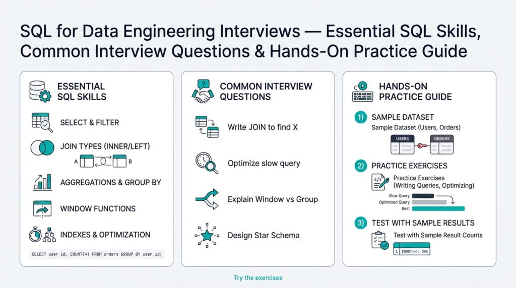
Hands-on interview practice problems
Building on this foundation, the fastest way to improve for SQL-based data engineering interviews is deliberate, hands-on practice problems that mirror production constraints. Start each session by picking a realistic schema and a performance goal—correctness first, then latency or bytes scanned—and iterate until your plan matches expectations. Practice problems should demand you reason about joins, window functions, aggregation, and physical design choices so you can explain trade-offs aloud during an interview. Treat each exercise as both a correctness challenge and a micro-benchmark for optimization.
Design practice problems that escalate in complexity: begin with data-cleaning tasks and deduplication, move to sessionization and time-windowed aggregates, then add scale concerns such as skewed joins and late-arriving rows. For example, create a dataset of event streams with duplicated event_ids, inconsistent user_ids, and an ingestion_time column that arrives late. Ask yourself to produce daily active users (DAU) and a 7-day rolling DAU while deduplicating on the latest ingestion_time. These constraints force you to combine CTEs, ROW_NUMBER(), and windowed aggregates in ways interviewers commonly probe.
Turn that prompt into a concrete query skeleton and iterate on it; here’s a compact pattern you’ll write in many interviews:
WITH dedup AS (
  SELECT *, ROW_NUMBER() OVER (PARTITION BY event_id ORDER BY ingestion_time DESC) rn
  FROM events
  WHERE event_ts >= DATE '2025-01-01'
)
SELECT event_date,
       COUNT(DISTINCT user_id) AS dau,
       SUM(COUNT(DISTINCT user_id)) OVER (ORDER BY event_date ROWS BETWEEN 6 PRECEDING AND CURRENT ROW) AS rolling_7d_dau
FROM (SELECT * FROM dedup WHERE rn = 1) t
GROUP BY event_date;
Write the simplest correct query first, then profile it with EXPLAIN/EXPLAIN ANALYZE to find dominant operators. Practice rewriting the same answer in three variants: one optimized for minimal scanned bytes (push filters, sargable predicates), one optimized for memory (pre-aggregate or broadcast small tables), and one resilient to late data (use LEFT JOINs or merge strategies). This pattern trains you to communicate a hypothesis—“I’ll push this predicate to reduce scanned partitions”—and then prove it with plan differences.
Scale-focused problems belong in every set. Simulate skew by duplicating a hot key and observe spill or skewed shuffle in the plan. Practice the salting technique to spread hot-key joins across N buckets: add MOD(ABS(HASH(key)), N) as salt to both sides, join on (key, salt), then re-aggregate. Also practice replacing exact distincts with sketches like HyperLogLog when acceptable, so you can argue a fidelity-versus-cost trade-off in an interview. These exercises teach you to measure bytes read, shuffle volume, and operator time rather than guessing what helped.
Finally, rehearse a crisp interview narrative: restate the problem, clarify constraints (freshness, exactness, SLA), present a correct baseline query, then show one targeted optimization and its measured effect. How do you choose between a GROUP BY and a window function under time and cost constraints? State the criteria, show the SQL, and point to the execution-plan metric that changed. By practicing this structure with realistic practice problems, you’ll be prepared to write maintainable, performant SQL and to explain the engineering trade-offs interviewers care about.