Indexing Fundamentals
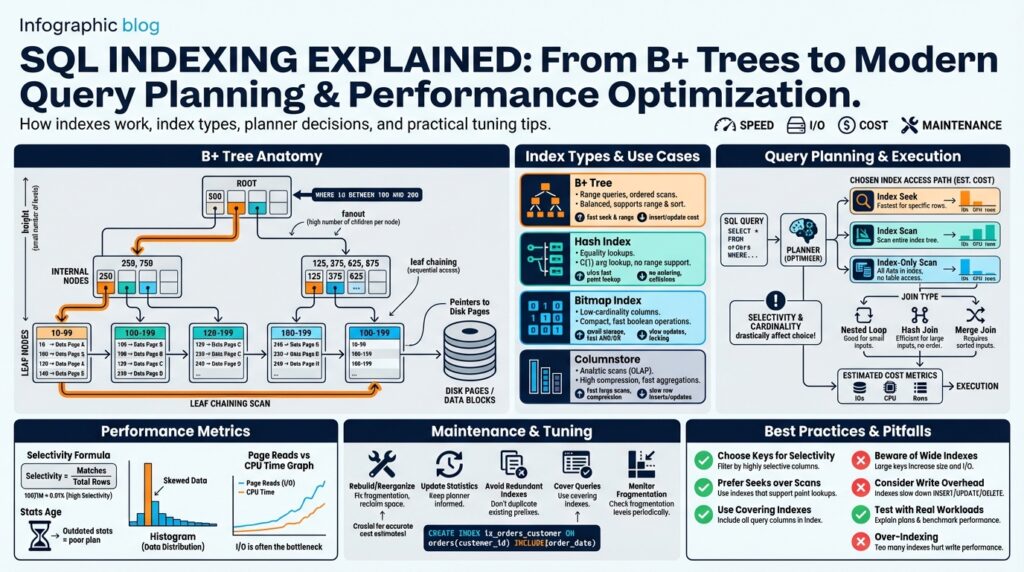
If your queries are slow, the first place to investigate is often SQL indexing, because an appropriate index turns expensive table scans into targeted lookups and directly impacts query planning and performance optimization. An index is a data structure that maps key values to row locations so the database can avoid reading every row; the dominant on-disk structure for range and ordered lookups is the B+ tree. A B+ tree is a balanced tree where internal nodes only store keys and leaf nodes store actual key-to-row pointers; this layout keeps tree height small and I/O predictable, which is why most relational systems rely on it for clustered and nonclustered indexes.
Building on this foundation, consider how indexes change the cost model of a query. A high-selectivity index—one where a predicate matches a small fraction of rows—lets the engine perform an index seek followed by a small number of random reads, whereas a low-selectivity index can lead to many random I/Os and sometimes a full table scan is still cheaper. For example, querying orders by an indexed unique order_id will be an index seek, but filtering by a boolean flag present in 90% of rows will likely be cheaper as a sequential scan. That selectivity calculus is exactly what the optimizer uses when comparing execution plans.
Not all indexes are equal; you must choose type and placement for the workload. A clustered index physically orders table rows by its key, which benefits range queries and ordered scans but ties the table to that ordering; a nonclustered index stores separate key-to-row mappings and can include additional columns (a covering index) to answer queries without touching the base table. Use a covering index when you can include the projected columns to avoid lookups—this reduces I/O and context switches between index and heap or clustered data.
Composite indexes introduce ordering and prefix rules you need to respect in practice. When you create an index on (A, B, C), the index is ordered by A then B then C, so queries must filter or sort on leftmost columns to benefit; predicates only on B and C won’t use that index efficiently. For multi-column equality and range mixes, place the most selective or most frequently filtered column first, and design the index to match typical WHERE, JOIN, and ORDER BY patterns. How do you choose the right index for a query? Start by examining the query predicates, join keys, and sort requirements, then model the selectivity and expected I/O.
Indexes improve reads but add write and storage costs—and that trade-off matters in OLTP systems. Each INSERT, UPDATE, or DELETE must maintain all relevant indexes, which increases commit latency and can cause write amplification and page splits in B+ trees; updates to indexed columns may incur a delete-and-insert in the index. We often avoid indexing low-selectivity columns, high-churn columns, or too many redundant composite permutations. In practice, monitor write latency and index maintenance metrics and prefer narrower keys (smaller width) to reduce tree depth and lock contention.
Finally, remember the optimizer is your partner: it relies on statistics about cardinality and distribution to decide whether an index is useful, and outdated statistics can mislead plan selection. Collect histograms and update stats after large data changes, and test with realistic workloads to see whether the planner uses a given index the way you expect. With these fundamentals—knowing how B+ trees work, matching index types to query patterns, balancing read/write costs, and feeding the planner good statistics—we can move into deeper internals of B+ tree node formats and how modern query planning leverages them for advanced performance optimization.
B+ Tree Structure Explained
Building on the foundation of SQL indexing, understanding the B+ tree at the byte-and-page level explains why an index turns expensive scans into predictable I/O patterns. The B+ tree is tuned for disk and SSD access: internal nodes act as a compact routing table while leaf pages contain the bulk of key-to-row pointers, so the tree’s fanout (entries per page) dominates height and lookup cost. If you want consistent seeks and efficient range scans, you need to think in pages, not just logical keys.
Internal nodes store only separator keys and child pointers, which keeps their size small and increases branching factor; leaf nodes store fully materialized entries (key plus row identifier or clustered row data) and are chained for sequential access. This separation reduces tree height because one internal entry can route to many children, and the sibling pointers on leaf pages enable low-cost forward/backward range iteration without touching parent nodes. Because internal nodes hold no payload rows, updates usually affect leaves first and only occasionally cause parent updates when splits propagate.
Fanout determines height, so make that calculation concrete when you design an index. For example, with an 8 KB page, an 8-byte key and an 8-byte pointer give an approximate entry size of 16 bytes; that yields a theoretical fanout around 8,192/16 ≈ 512 entries per node. For 100 million indexed rows that map to roughly 195,312 leaf pages, a two-level internal structure (root → level-1 → leaves) suffices: 195,312/512 ≈ 382 level-1 pages, and 382/512 ≈ 1 root page. The practical takeaway: wider keys reduce fanout, increase height, and multiply random I/Os for seeks—so prefer narrow index keys.
Operationally, a search descends internal nodes to a leaf, and an insert/update performs the same descent before modifying a leaf page in-place or splitting it if full. A split writes a new sibling, moves roughly half the entries, and inserts a separator into the parent; that parent may in turn split, cascading to the root and increasing tree height. Deletes can underflow a node and trigger redistribution or merge operations. These split/merge behaviors explain why high-churn columns and large composite keys increase write amplification and why fill-factor tuning matters to reduce hot page splitting.
Range scans are where the B+ tree really shines: because leaves are linked, a single index seek to the first matching leaf plus sequential reads of adjacent leaf pages produces a mostly sequential I/O pattern. How do you tune an index for range-heavy workloads? Place the most frequently ranged column as a leftmost key, keep keys compact to maximize entries per page, and consider a clustered index when the workload favors large ordered scans over random point lookups. Covering indexes still matter here: if the leaf stores all projected columns, the engine avoids lookups to the base table and your range scan remains index-local.
Taking this structure further, production databases layer optimizations on top of the basic B+ tree: prefix compression in leaf and internal node keys, adaptive page sizes, and concurrency-friendly latching schemes reduce storage and contention without changing the logical model. Next, we’ll examine specific node formats, compression choices, and how the optimizer uses page-level statistics to decide when an index seek, range scan, or full table scan makes the most sense.
Other Index Types Overview
Building on the B+ tree foundation we just covered, production systems commonly use several other index families to match specific access patterns and data shapes. These alternatives—hash indexes, bitmap indexes, inverted/full‑text structures, columnstore layouts, and spatial or generalized trees—aren’t replacements for B+ trees so much as complementary tools that change the cost model of your queries. Right up front: pick an index by how your queries access data (point lookups, range scans, multi‑valued predicates, or analytical scans), because choosing the wrong type can hurt both latency and write throughput. SQL indexing decisions become easier when you map each workload to the index family designed for it.
Hash indexes optimize equality lookups. If your common operation is WHERE id = ? or exact-match joins on high-cardinality keys, a hash index offers O(1) expected lookup cost and fewer pointer hops than a deep B+ tree. However, hash indexes do not support ordered range queries, so WHERE id BETWEEN ? AND ? cannot use them; they also require careful collision handling and can be less storage-efficient for some implementations. Use a hash index when you need extremely fast point queries and you rarely sort or range-scan on that column; otherwise the B+ tree’s range abilities will be more useful.
Bitmap indexes excel for low-cardinality or boolean-like columns in read-heavy analytic workloads. A bitmap index represents each distinct value as a compressed bitset over row positions, making complex predicate combinations—WHERE country = 'US' AND active = true—very cheap through bitwise AND/OR operations. When should you use a bitmap index versus a B+ tree? Choose bitmap indexes for large, mostly‑static tables where many filters combine and updates are rare, because frequent DML causes bitmap maintenance costs and concurrency overhead. In data warehousing queries that aggregate across many filters, bitmap indexes often beat tree scans by orders of magnitude.
Inverted and generalized indexes handle multi-valued and unstructured data. An inverted index maps tokens (words, JSON keys, array elements) to posting lists of row identifiers, which is why search engines and full‑text search features rely on them. In systems like PostgreSQL, GIN (Generalized Inverted Index) is tailored for indexing arrays, JSONB keys, and full-text tokens, while GiST (Generalized Search Tree) provides an extensible framework for range, nearest‑neighbor, and custom operators. If you index nested JSON fields or text columns and your queries ask “which rows contain this token?” an inverted/Gin index will often be the right tool.
Columnstore indexes (columnar storage) flip the row layout to optimize analytic scans. By storing each column contiguously and applying compression, columnstores reduce I/O for wide tables when queries project a small subset of columns and perform aggregations or sequential scans. Vectorized execution engines paired with columnstore indexes amplify these gains by processing many values per CPU cycle, but expect higher latency for single‑row lookups and complexity in maintaining up-to-date data with frequent point writes. For OLAP workloads and nightly batch reports, columnstore delivers dramatic storage and scan performance improvements compared with row‑oriented B+ tree indexes.
Specialized spatial and multi-dimensional indexes—R-trees, KD-trees, and their variants—solve geometric queries like bounding‑box searches and nearest neighbors. These structures prioritize spatial locality and overlap testing rather than strict key ordering, so they power queries such as ST_DWithin(geom, point, radius) efficiently. When you design geospatial features or multi‑attribute nearest‑neighbor search, use these spatial indexes and tune parameters (node fanout, bounding heuristics) to balance tree depth and overlap.
Choosing among these families is an engineering trade-off: point vs range, static vs high‑churn, single‑valued vs multi‑valued, and transactional vs analytic. We recommend profiling representative queries, measuring index maintenance cost during realistic write patterns, and validating optimizer plans with live statistics. With that empirical feedback loop—test plans, update stats, and monitor I/O—you can combine B+ trees, hash indexes, bitmap indexes, inverted and columnstore structures to cover the full spectrum of production workloads and let the optimizer pick the most efficient access path for each query.
How Query Planner Uses Indexes
Building on the B+ tree and selectivity discussion from earlier, the query planner is the engine that maps logical predicates to concrete index access paths and compares their I/O cost against alternatives. In practice, the planner operates as a cost-based decision-maker: it estimates the number of rows a predicate will return, converts that cardinality into expected page reads and CPU work, and then chooses between an index seek, a range scan, an index-only (covering) scan, or a full table scan. Because these cost estimates drive production latency, understanding how the planner interprets your indexes gives you leverage to shape plans rather than reacting to them.
How does the planner decide between an index seek and a table scan? The short answer is selectivity plus I/O cost modeling: the planner multiplies estimated qualifying rows by the per-row random I/O (for non-sequential leaf reads) and compares that against the sequential scan cost for reading whole pages. It uses statistics—histograms, distinct count, null frequency—to estimate selectivity for predicates, and it factors in page-level locality and clustering (a clustered index reduces random reads for range queries). When selectivity is high, an index seek plus a few lookups wins; when selectivity is low, a table scan often remains cheaper.
The planner exposes several concrete access paths and will choose the one with the lowest projected cost. For point lookups (for example, queries like SELECT * FROM orders WHERE id = ?), the planner favors an index seek that walks the B+ tree to the leaf and fetches the row directly. For ordered ranges (SELECT … WHERE ts BETWEEN ? AND ? ORDER BY ts) it prefers a range scan that starts at the first matching leaf and reads adjacent pages sequentially, which leverages leaf chaining for efficient forward iteration. If the leaf entries already contain all projected columns, the planner can produce an index-only or covering scan that avoids base-table lookups and dramatically reduces I/O and context switches.
Indexes also change join and sort strategies in measurable ways. When a join uses a highly selective index on the inner table, the planner may choose a nested-loop join and perform an index lookup per outer-row; conversely, if no suitable index exists or estimated output is large, it will prefer a hash or merge join to avoid repeated random reads. Similarly, an index ordered on the ORDER BY columns can allow the planner to skip an explicit sort phase—saving CPU and memory—by producing rows already in the required order. These decisions depend on join cardinality estimates, index key ordering, and whether the index is clustered or nonclustered.
Beyond single-index choices, modern planners use composite techniques that combine indexes and statistics. Index intersection (also called index merge) can satisfy conjunctive predicates by reading two smaller indexes and intersecting their row-id results when no single covering index exists. Bitmap and compressed index structures let the planner perform fast bitwise operations for highly selective multi-predicate analytics. The planner also respects partial and expression-based indexes, applying predicate pushdown to check whether an index’s filter condition matches the query; that makes partial indexes powerful for skewed, hot subsets of data. Finally, adaptive features—runtime re-optimization, parameter sniffing, and feedback-based cardinality correction—help the planner recover when static statistics mispredict runtime distributions.
To influence plan selection effectively, update and shape the planner’s inputs rather than guessing at its internals. Keep statistics fresh after major data changes, add covering or partial indexes for hot queries, and validate expected plans with EXPLAIN ANALYZE under representative data and parameter distributions. When you must force behavior, use hints sparingly and only as a last resort; instead, iterate on narrower keys, include frequently projected columns in leaf entries, and measure write cost as you add indexes. By treating the query planner as a cost engine that reacts to selectivity, page locality, and index payload, you can design indexes that the planner will actually choose—and that will deliver predictable performance for your workload.
Designing Effective Indexes
If your production queries still stall after adding indexes, the problem is often index design rather than the absence of an index. Early in your troubleshooting workflow, treat SQL indexing as a deliberate modeling decision: the index key shapes B+ tree fanout, leaf density, and ultimately whether the query planner chooses a seek, range scan, or table scan. We need compact, workload-aligned keys that reflect how your queries filter, join, and sort; otherwise the optimizer will ignore the index and you’ll pay for storage and maintenance without read-side benefit.
Choose index keys by mapping them to real query patterns and cardinality distributions rather than convenience. Start with the predicates and ORDER BY clauses you see in EXPLAIN plans, then prefer the most selective or most frequently filtered column as the leftmost key in a composite index; for instance, an index on (user_id, created_at) benefits per-user range scans, while reversing that order defeats the left-prefix rule. Include frequently-projected but low-selectivity columns as cover-only payloads (for example, INCLUDE (status, total) in systems that support included columns) so the B+ tree leaf contains all columns the planner needs and avoids lookups to the base table.
Design covering indexes strategically because they change the cost model from random lookups to index-only scans. A covering index stores projected columns in leaf pages so a single range scan returns fully materialized rows from the index; that reduces context switches and random I/O but increases key width and reduces fanout in the B+ tree. Balance this by keeping keys narrow and pushing non-key payload into INCLUDE columns when possible; wider leaf payloads raise tree height and per-seek I/O, so measure the change in index pages and average depth before deploying broadly.
Use partial and expression-based indexes to capture hot subsets or computed predicates without indexing the whole table. When should you use a partial index? Apply it when a small, high-impact subset of rows drives most queries—e.g., WHERE status = 'active' for active-user reports—so the planner can use the smaller index for those queries while avoiding write amplification for the rest of the table. Expression indexes (indexing lower(email) or a JSON path) convert runtime computations into sargable access paths that the query planner can match directly, but remember to keep statistics and query forms aligned so the planner recognizes the index.
Account for write-side cost and concurrency from the start: every additional index is a synchronous maintenance step on INSERT, UPDATE, and DELETE. Tune fill-factor to trade empty space for fewer page splits under heavy insert workloads, and avoid indexing high-churn, low-selectivity columns that will amplify write latency and fragmentation. Monitor index health via EXPLAIN ANALYZE for hot queries and your RDBMS’s usage views (index usage DMVs or equivalent) to discover unused or redundant indexes, then iterate: remove, consolidate, or rebuild based on real maintenance and latency metrics rather than intuition.
Treat index design as an iterative optimization loop: design, deploy under a representative dataset, validate with EXPLAIN ANALYZE and latency percentiles, then refine keys, includes, and fill-factor. We should also update statistics after bulk changes so the query planner has accurate cardinality inputs and will choose the index the way we expect. By grounding index choices in query patterns, B+ tree fanout considerations, and measured trade-offs between read improvement and write overhead, you create indexes that the planner will use and that produce stable, predictable performance as your workload evolves.
Index Maintenance and Monitoring
Indexes wear out: they fragment, statistics drift, and usage patterns change as your application evolves. Building on the B+ tree and planner concepts we covered earlier, proactively prioritizing index maintenance and index monitoring keeps query latency predictable and prevents the optimizer from making poor choices. You should treat maintenance as part of the index lifecycle—not an occasional chore—because stale statistics or a fragmented leaf layer convert well-designed SQL indexing into a performance liability.
Start by instrumenting the right signals: track index usage counts, page-level fragmentation or bloat, statistics staleness, page-split frequency, and index size growth. Fragmentation (noncontiguous logical ordering of leaf pages) increases random I/O for seeks and range scans; bloat or dead tuples increase the number of pages the planner thinks it must read. Statistics staleness leads the planner to misestimate selectivity and choose suboptimal plans; we define “stale” when the row distribution or distinct counts change substantially after bulk loads, deletes, or high-churn updates.
When you detect problems, apply the correct remediation: reorganize for light fragmentation, rebuild for severe fragmentation or compacting bloat, and update statistics after major DML. A reorganize performs in-place compaction with minimal locks, reducing fragmentation gradually, while a rebuild creates a new index structure and drops the old one—often reducing height and improving fanout but incurring higher I/O and potential locks unless your engine supports online rebuilds. Tune fill-factor to trade free leaf-space for fewer page splits under heavy insert patterns: lower fill-factor reduces splits but increases index size, so measure write amplification and depth after changes.
Operationalize maintenance with rules and windows that reflect your workload characteristics. For largely read-only analytic tables, schedule off-peak full rebuilds and aggressive compression; for high-throughput OLTP tables, prefer incremental reorganize or online rebuild with throttling to avoid impacting commit latency. Avoid blanket weekly rebuilds—automated jobs should be driven by metrics (e.g., fragmentation > X% and writes per second > Y). We also recommend performing maintenance on replicas first when possible, then switching roles to avoid production downtime while validating the new index footprint and plan behavior.
Make your monitoring actionable by capturing both engine-specific and generic signals and surfacing them in dashboards and alerts. For example, query engine usage views to find unused indexes and heavy-maintenance candidates: in SQL Server you can join sys.indexes with sys.dm_db_index_usage_stats to see seeks/scans/updates, and in PostgreSQL use pg_stat_user_indexes and pg_statio_user_indexes to observe index scans and heap fetches. Instrument latency percentiles and I/O per query alongside index usage so you can correlate a spike in 99th-percentile latency with rising page-splits or an index having many updates per second.
How do you validate that maintenance improved performance? Always measure before-and-after with representative workloads: run EXPLAIN ANALYZE or equivalent on the same queries, capture end-to-end latency percentiles, and compare IO metrics like random reads/sec and bytes read. Avoid relying solely on index size reduction as success—sometimes a smaller index increases CPU due to decompression; the ultimate judge is query throughput and tail latency under production-like concurrency.
Finally, embed index maintenance into your change pipeline and feedback loop so it evolves with schema and workload changes. Revisit partial and covering index choices when usage patterns shift, refresh statistics after bulk loads, and automate alerts for unexpected growth or unused indexes. By combining continuous index monitoring, targeted maintenance actions, and empirical validation, we keep SQL indexing and B+ tree structures tuned for stable, predictable query planning and real-world performance.