Logical vs Physical Order
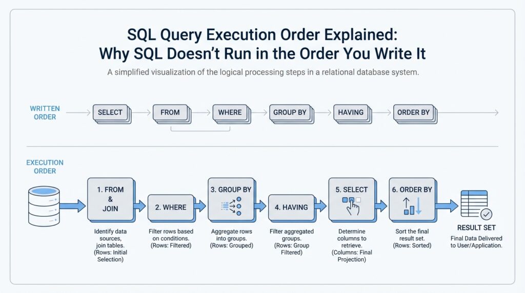
Building on this foundation, the first thing to separate is the story your SQL statement tells from the work the database actually performs. The logical query processing order is the educational model that says the engine reasons through a query in stages such as FROM, JOIN, WHERE, GROUP BY, HAVING, SELECT, and ORDER BY. That model helps you understand why a clause can only see certain names or values at a given moment. When you feel SQL is “ignoring” the order you typed, it is usually following that logical order rather than the line-by-line layout on the page.
Physical execution order is different. Once the optimizer has understood your query, it builds a query plan, which is the engine’s roadmap for fetching rows, joining tables, filtering data, sorting results, and sometimes skipping work with indexes. PostgreSQL says there are many possible ways to execute the same query, and the planner chooses the one it expects to run fastest; MySQL’s EXPLAIN shows how the optimizer will process the statement, including join order. The key idea is that the physical path can change while the final result stays the same.
That is why EXPLAIN is such a useful flashlight. It shows you the plan instead of the prettified SQL, so you can see whether the database scans a table, uses an index, or reorders joins to reduce work. In PostgreSQL, EXPLAIN displays the plan tree the planner creates; in MySQL, it reveals the optimizer’s execution plan and join order, and it can even help you spot where an index would speed things up. If two queries return the same answer but one is much slower, the difference is often in the physical execution order, not in the logical meaning of the statement.
This difference matters most when you mix filtering and aggregation. Suppose you write a query like SELECT department, SUM(salary) AS total_salary ... and then try to filter on total_salary in WHERE. You are asking for a value that does not exist yet in the logical query processing order. MySQL’s manual says standard SQL disallows column aliases in WHERE because the alias is not known until after rows are selected and grouped, while Microsoft’s SQL Server tools show that HAVING is applied after grouping and is the place for conditions that depend on aggregated results. That is why a beginner’s query may look reasonable on the page but still fail at runtime.
Once you start thinking in terms of logical vs physical order, SQL feels less like a trick and more like a conversation with a very efficient assistant. You describe what you want, the logical order explains what each clause is allowed to see, and the physical execution order shows how the database gets the job done. The optimizer is free to change the route, but it must preserve the same result set, which is why well-written queries can be both readable and fast. With that in mind, the next step is to look at how individual clauses behave inside that larger story.
Start with FROM
Building on this foundation, the first room we walk into is FROM, because SQL query execution order has to know where the rows come from before it can do anything else. Think of it like opening a map before choosing a route: the database needs a source table, view, subquery, or function to build the working set. PostgreSQL describes the FROM list as the intermediate virtual table that feeds the rest of the query, and it says the later WHERE, GROUP BY, and HAVING clauses all transform that table in sequence.
That is why FROM feels less like a decorative opening line and more like the stage crew. It names the tables, can assign aliases, and can even join multiple sources into one row set. Once an alias exists, the rest of the query uses that new name, not the original one, which is why a WHERE clause must reference the alias if one was given. PostgreSQL also allows subqueries, VALUES lists, and table functions in FROM, so the clause can be much richer than a single table name.
Why does SQL start with FROM? Because the database cannot filter, group, or label rows until it has row sources to work with. If you picture a query like a recipe, FROM is the ingredient list and the first prep step at the same time: it tells the engine what raw material exists, how those pieces relate, and what the combined table should look like before anything else happens. PostgreSQL even notes that LATERAL subqueries can look back at earlier FROM items, which is another clue that this clause is the place where the row set is assembled, one source at a time.
This is where the SQL query execution order starts to feel concrete. When you write a join, FROM is where the database decides which tables participate and how they line up, while ON describes the match condition for the join itself. PostgreSQL points out that an inner-join restriction can live in either ON or WHERE, but a restriction in ON is processed before the join and the same restriction in WHERE is processed after the join; with outer joins, that difference matters a lot. So if a query seems to “move” rows around, the truth is that FROM built the joined row set first, and the later clauses are working on that result.
Once you see FROM as the starting point, the rest of the logical query processing order becomes easier to trust. WHERE is not the place where rows are born; it is the place where rows are accepted or rejected after FROM has already created the working table. That same idea is why aggregate questions feel tricky in beginner SQL: GROUP BY and HAVING only make sense after the row source exists, because they operate on rows that FROM has already gathered. In practice, reading a query from FROM forward helps you answer a simple but powerful question: what data exists at this moment, and what clauses are allowed to see it?
Join Tables First
Building on this foundation, the next thing to picture is the moment two tables meet. In SQL query execution order, the database does not wait until the end to decide how rows relate; it starts by building a joined row set inside the FROM clause so later clauses can work with one combined result instead of separate tables. PostgreSQL describes a joined table as being derived from two tables, and it notes that JOIN clauses can nest, with left-to-right grouping unless you add parentheses to change the order.
That is why the join condition matters so much. Think of ON as the matching rule, like telling a librarian which book card belongs with which shelf label, before we decide whether the pair should stay in the final display. PostgreSQL says ON is the most general kind of join condition and that two rows match when the ON expression is true; MySQL adds that ON usually describes how tables join, while WHERE limits which rows survive in the result. What happens when you blur those two jobs together? That is where a lot of beginner confusion starts.
For inner joins, this separation is mostly a readability choice, because the same match can often be written in JOIN/ON or in WHERE and still produce the same rows. PostgreSQL’s tutorial shows that the older comma style with a WHERE comparison and the newer explicit JOIN/ON form are equivalent for that kind of join, which is why the explicit form is easier to read without changing the result. When tables arrive in threes or fours, parentheses become the road signs: PostgreSQL says joins can be chained or nested, and without parentheses they associate left-to-right, so each partial result is built step by step before the next table joins in. Once you see that, SQL query execution order feels less mysterious: JOIN is where the pairing happens, and WHERE is where the already-paired rows are checked.
Outer joins are where the story changes. A LEFT JOIN keeps every row from the left table even when there is no match on the right, and the missing side is filled with nulls, which is SQL’s way of saying there was no partner here. PostgreSQL explains that an outer join first performs the match and then adds rows for the unmatched side, and MySQL shows the same pattern by returning NULLs for missing right-table columns. If you move a condition that belongs in ON into WHERE, you can accidentally remove those preserved rows and make the join behave like a stricter filter than you intended.
A helpful way to read a join is to ask two questions in order. First, what relationship is the database creating between these tables? Then, which rows should still survive even when no match exists? That mental pause is useful because JOIN tables first is not about memorizing a rule; it is about seeing that the database builds a shared row space before later clauses inspect it. In that sense, the join becomes the bridge, not the destination.
Keep that bridge image in mind as you read more complex queries. Once the join has created the combined row set, later clauses can filter, group, or sort it, but they are working with the joined result, not with the original separate tables. That is why the SQL query execution order starts to feel calmer when you treat joins as the first act of the scene: the database is assembling the cast before the rest of the story can unfold.
Filter Rows with WHERE
Building on this foundation, WHERE is the part of SQL query execution order where rows get their first real test. After FROM has gathered the working table and joins have stitched tables together, WHERE acts like a gatekeeper: it looks at each row and decides whether that row should continue or be filtered out. If you have ever wondered, “How do you filter rows in SQL without changing the meaning of the rest of the query?” this is the clause that answers that question.
The key idea is that WHERE evaluates a condition, called a predicate, which is a test that returns true, false, or unknown. That last outcome matters because SQL treats NULL as missing or unknown data, not as zero or an empty string. So when a row contains NULL in a column used by WHERE, the condition may not become true even if it looks close enough at first glance. In practice, WHERE does not try to fix the data or interpret your intention; it only asks, “Does this row satisfy the rule I was given?”
That makes WHERE feel a lot like a sieve. The rows already exist by the time the clause sees them, and the filter simply lets some pass through while holding others back. You might write a condition like salary > 50000, department = 'Sales', or created_at >= '2026-01-01', and each one narrows the result to the rows that match your search. This is why WHERE is so often the first tool you reach for when you want a smaller, cleaner result set rather than a summarized one.
Because WHERE works after the row source is built, it can combine several tests in one place. You can stack conditions with AND when every rule must be true, OR when any one rule can qualify, and NOT when you want to exclude a pattern. The important part is that SQL evaluates the rows that FROM produced, not the labels you may add later in SELECT, which is why a fresh alias usually cannot be used in WHERE. Once that timing clicks, the clause stops feeling mysterious and starts feeling predictable.
This timing also explains one of the most common beginner surprises: WHERE can remove rows before later stages ever see them. If you are working with an outer join, a condition placed in WHERE can accidentally discard the unmatched rows that the join was supposed to preserve. That is why careful SQL writing is less about memorizing syntax and more about understanding where each rule belongs in the flow. When you want to keep unmatched rows, you need to think about whether a condition belongs in the join logic or in the row filter.
A helpful way to picture the difference is to imagine a restaurant kitchen. FROM gathers the ingredients, joins combine matching ingredients into one dish, and WHERE is the taste test that says which plates are good enough to serve. If a plate fails the test, it never reaches the table, but nothing about the plate itself is changed. That is what makes WHERE so powerful: it is selective, not transformative.
Once you see WHERE as the row filter in SQL query execution order, a lot of other behavior starts to make sense. You understand why it comes before aggregation, why it cannot rely on values that have not been created yet, and why it can silently shape the meaning of a join. That same mental model will help us as we move forward, because every later clause builds on the rows that have already survived this first pass.
Group Rows with GROUP BY
Building on this foundation, GROUP BY is the moment when SQL stops looking at rows one by one and starts asking, “Which rows belong together?” After WHERE has trimmed the working set, GROUP BY gathers the survivors into buckets that share the same value in one or more columns. Think of it like sorting receipts into envelopes by month, department, or customer before you add anything up. In SQL query execution order, that step matters because aggregation cannot happen until the rows have been collected into meaningful groups.
So what does GROUP BY do in practice? It turns many detailed rows into fewer summary rows, with one output row for each group. If you group sales by department, then all sales rows for Marketing become one basket, all rows for Engineering become another, and so on. That is why GROUP BY often appears beside aggregate functions such as SUM (which adds values), COUNT (which counts rows), AVG (which finds the average), MIN (which finds the smallest value), and MAX (which finds the largest value). Once you see it this way, GROUP BY feels less like a syntax rule and more like a sorting step before the math begins.
Here is where things get interesting: the database needs to know exactly what counts as “the same group.” If you write GROUP BY department, then each distinct department becomes its own group, and the aggregate function works inside that group only. A query such as SELECT department, SUM(salary) FROM employees GROUP BY department means, “Show me one row per department, and give me the total salary inside each department.” That is the core idea behind grouping rows with GROUP BY: you are not changing the original data, you are telling SQL how to organize it so it can summarize it cleanly.
Why does SQL complain when you select a column that is not grouped or aggregated? Because one group contains many rows, and SQL needs one clear answer for each column in the result. If the group contains five different employee_name values, which one should the database show? It cannot guess, so most databases require every non-aggregated column in the SELECT list to be part of the GROUP BY clause. This rule is one of the biggest mental shifts for beginners, but it makes sense once you remember that a grouped query returns one row per group, not one row per original record.
A helpful way to picture GROUP BY is to imagine a classroom attendance sheet. First, we separate students by homeroom, and only then do we count how many students are in each room or calculate the average score in each room. The grouping comes before the summary, just like sorting ingredients comes before cooking a sauce. In the same way, SQL query execution order uses GROUP BY to build the containers first, then applies the aggregate logic inside each container. That is why grouped queries can answer questions like “How many orders came from each city?” or “What is the total revenue per product line?” without forcing you to scan the rows manually.
This timing also explains why GROUP BY feels different from WHERE. WHERE filters individual rows before they are grouped, while GROUP BY reshapes the row set into summaries after the filter has done its work. In other words, WHERE decides who gets into the room, and GROUP BY decides how the guests are seated once they are inside. If you are trying to understand SQL query execution order, this is a useful checkpoint: by the time grouping happens, the database already knows which rows remain, and it is ready to combine them into a smaller, more meaningful result set.
Once that clicks, grouped queries stop feeling mysterious and start feeling deliberate. You are not asking SQL to “magically” total data; you are telling it how to bundle rows so the totals make sense. That same idea prepares us for the next step, because once the groups exist, we can decide which groups deserve to stay and which ones should be filtered out.
Filter Groups with HAVING
Building on this foundation, HAVING is where grouped data gets its final test. After WHERE has trimmed rows and GROUP BY has bundled them into summaries, HAVING decides which summaries stay in the result. If WHERE is a sieve for individual rows, HAVING is the inspector standing at the door of each bucket of rows. That difference is the heart of SQL query execution order, and it is why a query can look correct while still failing if you place a group-level condition in the wrong clause.
The easiest way to see it is with a departmental salary report. Suppose we group employees by department and calculate total salary or average salary. We are no longer asking about one employee at a time; we are asking about the group as a whole. HAVING lets you say, “Show me only the departments whose total salary exceeds 1,000,000,” or “Keep only groups with more than 10 employees.” That is a group filter, not a row filter, because the answer depends on the aggregation itself.
Why not use WHERE for that job? Because WHERE runs before aggregation, so it can only inspect raw rows that exist before the groups are formed. A condition like salary > 1000000 would test each employee’s salary, which is a very different question from testing the total salary of an entire department. This is the same timing rule we have been building on throughout SQL query execution order: each clause can only see the data that already exists at that point in the story.
Once that clicks, HAVING stops feeling like a special trick and starts looking like a post-group checkpoint. The database first creates the groups, then it evaluates the HAVING condition against each group, and only then does it hand the surviving groups to SELECT for display. If you have ever wondered, “Why does my query return fewer departments than I expected?” the answer is often that HAVING quietly removed the groups that did not meet the threshold. The result is not random; it is the outcome of a filter that works on summaries.
A useful mental model is a classroom awards night. WHERE decides which students are eligible to be counted, GROUP BY sorts them into classes, and HAVING decides which classes deserve recognition after the averages or totals are calculated. That is why SQL query execution order matters so much when you write reporting queries. You are not just listing steps on a page; you are guiding the database through a sequence where each stage depends on the last one.
In practice, the HAVING clause often appears with aggregate functions such as COUNT, SUM, AVG, MIN, and MAX, because those functions produce the numbers that make a group-level decision possible. For example, HAVING COUNT(*) >= 5 keeps only groups that have at least five rows, while HAVING AVG(score) > 80 keeps only groups with a strong average. The details of syntax can vary slightly across databases, but the role stays the same: HAVING filters grouped results after aggregation has done its work.
That timing also explains a common source of confusion with aliases and computed values. A name you create for a summary may feel visible everywhere, but the database still follows the logical sequence, so the group has to exist before it can be judged. When you read a query from FROM through HAVING, the path starts to feel steady instead of magical: rows are gathered, filtered, grouped, and then tested as groups. With that pattern in mind, you can look at a report query and ask the right question at the right moment: am I filtering rows, or am I filtering groups?
Sort Results with ORDER BY
Building on this foundation, we finally reach the moment when the result set becomes readable. ORDER BY is the clause that sorts results, and it comes after the database has already gathered, filtered, grouped, and sometimes reduced the rows. Think of it like arranging a stack of finished index cards after the research is done: nothing new is being created, but the order now helps you make sense of what you have. If you have ever asked, “How do you sort results in SQL without changing the data itself?” this is the clause that answers that question.
The important thing to notice is that ORDER BY changes presentation, not meaning. Earlier clauses decide which rows survive; ORDER BY decides which surviving row appears first, second, or last. That is why a query can return the same records in a different order when you add ORDER BY salary DESC or ORDER BY department ASC, last_name ASC. The rows are not altered, and the totals are not recalculated; we are simply telling SQL how to line them up for the final view.
Once that clicks, the clause starts to feel much less mysterious. ASC means ascending order, which usually means smallest to largest or A to Z, while DESC means descending order, which reverses that direction. You can sort on one column or several, and SQL will use the first sort key, then break ties with the next one, much like sorting a pile of mail first by zip code and then by street name. That same logic makes ORDER BY especially useful after GROUP BY, because you can sort summaries by the largest total, the highest average, or the most recent date.
Here is where the timing matters in SQL query execution order. ORDER BY sees the output of the query at the end of the logical pipeline, so it can sort raw rows, grouped rows, or calculated columns that already exist by the time sorting begins. If you write a report with SUM(sales) and then order it by that total, the database first builds the summary and then arranges the finished rows. That is why ordering a grouped report feels natural: we are not asking SQL to sort pieces that do not exist yet; we are sorting the completed answer.
You may also notice that ORDER BY is the place where search results often become useful to humans. Without it, SQL is free to return rows in whatever physical order happens to be convenient, which can look random from one run to the next. With it, you give the database a clear instruction about what “first” means. In practice, that is how you build lists like newest orders first, top-scoring students first, or alphabetized customer names, and it is why ORDER BY is so common in reports, dashboards, and paginated views.
One subtle detail is that sorting can involve values that are not obvious at first glance. A column can contain NULL, which means missing or unknown, and databases may place those values at the beginning or end depending on the system and the direction of the sort. That is one more reason to be explicit when the order matters to your reader. When you want a predictable result, ORDER BY gives you the final polish: it takes the answer your query has already built and arranges it into the sequence you actually want to see.