Why Optimize SQL?
Poorly performing SQL directly harms applications: slower page loads, unhappy users, missed SLAs, higher infrastructure bills, and database contention under load. Optimizing queries reduces latency, cuts I/O and CPU usage, improves concurrency, and lets the same hardware support more traffic and analytical workload with fewer trade-offs. Small changes—adding the right index, pushing filtering into the database, selecting only needed columns, or rewriting an inefficient join—often convert multi-second responses into milliseconds and drop scan-heavy I/O by orders of magnitude.
Beyond raw speed, optimization improves predictability and reliability. Stable, efficient queries reduce lock waits and timeouts during traffic spikes, make backups and maintenance windows shorter, and simplify capacity planning. For teams, fewer performance incidents mean faster feature delivery and less firefighting.
Start by measuring: capture execution plans, collect query latency and I/O metrics, and rank queries by total cost (frequency × latency). Fix high-impact offenders first: add selective indexes, avoid functions on indexed columns, replace cursor/N+1 patterns with set-based operations, and keep statistics up-to-date. These targeted improvements deliver the biggest business and technical gains with the least effort.
Reading Execution Plans
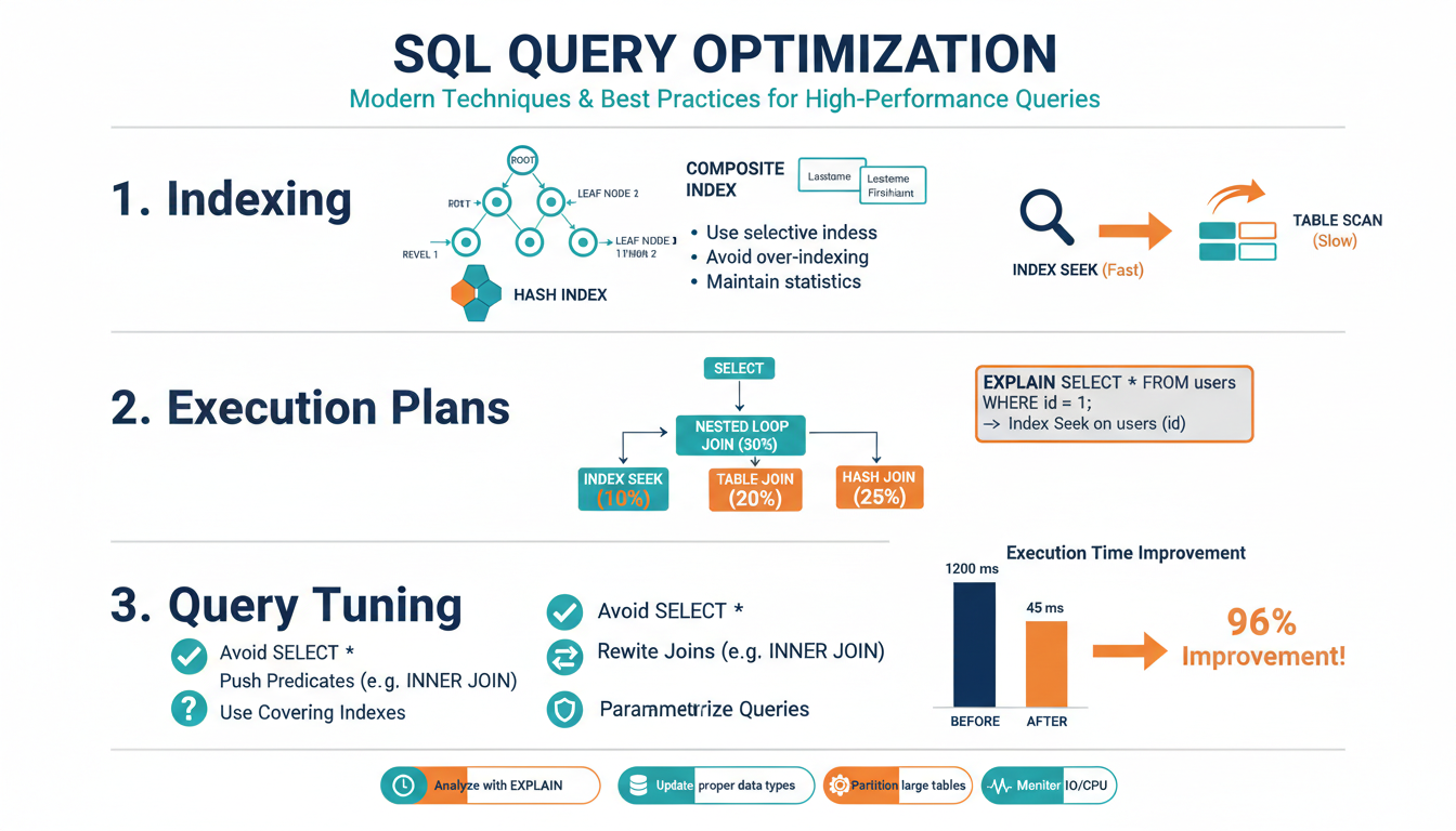
Begin by locating the operator tree and reading it from the data-access leaves upward toward the root—leaf nodes show scans/seeks, middle nodes show joins/sorts/aggregations, and the root is the final output. Focus first on the operators that consume the highest percentage of total cost; they are the best optimization targets. Compare estimated vs actual rows: large discrepancies point to stale or insufficient statistics, parameter sniffing, or inaccurate cardinality estimates and are often the root cause of a bad plan. Inspect access methods: an Index Seek on a selective predicate is usually good; an Index Scan or Table Scan on a selective filter suggests a missing or non-covering index. For joins, recognize Nested Loops (good for small inner inputs), Hash Match (used for larger, non-indexed joins), and Merge Join (requires sorted inputs or useful indexes); choose remedies based on which operator is costly. Watch for expensive sorts and spills to temp space (indicates insufficient memory or missing indexes), and for parallelism or Exchange operators that add coordination overhead. Pay attention to warnings and missing-index suggestions provided by the engine, but validate them—auto-suggested indexes can help but may not be optimal for workload. Use the plan’s IO/CPU breakdown and actual runtime stats (EXPLAIN ANALYZE / actual execution plan) to prioritize fixes: update statistics, add targeted composite or covering indexes, rewrite predicates to allow index use (avoid functions on indexed columns), and reduce row counts early with pushed-down filters. Iterate: after each change, capture a new plan and confirm reduced cost, lower I/O, and closer estimated-to-actual row alignment.
Indexing Fundamentals
Indexes are the primary lever for turning scan-heavy queries into fast seeks, but they’re a tradeoff: each index speeds reads and adds storage and write overhead. Choose indexes that reduce I/O on your highest-cost, highest-frequency queries rather than indexing every column.
Favor B-tree (balanced) indexes for range and equality predicates; use clustered indexes to define table order when most queries benefit from that ordering, and nonclustered indexes for additional access paths. Create composite indexes using the most selective, most-used predicate first (left-most prefix matters). Use covering indexes—add non-key INCLUDE columns—to avoid lookups: CREATE INDEX ix_orders_user_date ON orders(user_id, order_date) INCLUDE(total_amount).
Filtered indexes can dramatically reduce index size and maintenance when predicates are selective to a subset (e.g., WHERE deleted = 0). Avoid indexing columns that are frequently updated, and never rely on functions on indexed columns (col + 0 or LOWER(col) prevents index use); instead rewrite predicates or use computed, persisted columns where supported.
Keep statistics current and monitor fragmentation and index bloat; set sensible fillfactor for write-heavy indexes and schedule rebuilds/reorganizes based on fragmentation and resource windows. Regularly remove unused indexes by correlating index usage DMV data with query plans.
Always validate changes with actual execution plans and metrics: confirm a seek replaced a scan, I/O and CPU dropped, and estimated vs actual row counts tightened. Iterate—add the minimal, targeted index that yields measurable cost reduction.
Statistics & Cardinality Estimation
Accurate row-count estimates are the single biggest lever for stable, low-cost plans. Database optimizers rely on table and column statistics (histograms, distinct-value counts, null fractions, density) to predict how many rows a predicate or join will produce; large estimation errors cascade through join choice, join order, and operator selection, often turning seeks into expensive scans or causing memory spills. Start by comparing estimated vs actual rows using EXPLAIN ANALYZE or the engine’s actual execution plan to spot large discrepancies. When estimates are wrong, refresh or rebuild statistics with a full scan or increased sampling; enable and tune automatic statistics where safe, and schedule manual updates after bulk loads, ETL jobs, or major data-skew changes. For correlated predicates, create multi-column/extended statistics or use persisted computed columns so the optimizer sees joint distributions. For partitioned tables, use incremental statistics or per-partition stats to avoid stale, averaged estimates. Filtered stats are valuable when a small subset dominates queries (e.g., active = 1). Be cautious with parameter sniffing: if parameter variability causes bad plans, consider plan-parameterization strategies, plan guides, or recompilation hints sparingly. Finally, validate every change by capturing a new plan and workload metrics: tighter estimated-to-actual ratios should reduce IO/CPU and change costly operators to seeks, merge joins, or more efficient join orders. Treat statistics tuning as part of regular performance maintenance, not a one-off task.
Query Rewriting Techniques
Start by making predicates SARGable: move functions off indexed columns (rewrite WHERE LOWER(name) = 'alice' to WHERE name = 'Alice' or use a persisted computed column) and avoid implicit conversions that force scans. Push filters as early as possible—apply selective WHERE clauses in derived tables or JOIN conditions so row counts shrink before expensive operations. Replace OR-heavy predicates with UNION ALL or indexed IN lists when each branch can use an index, and prefer EXISTS over IN for correlated subqueries when duplicate suppression isn’t required. Convert correlated subqueries and row-by-row logic into set-based operations or JOINs; where a correlated subquery is unavoidable, use LATERAL/CROSS APPLY (or the engine’s equivalent) to express efficient, planner-friendly access. Swap cursors and procedural loops for window functions and batch aggregates—ROW_NUMBER() or RANK() often replace self-joins used for top-N-per-group patterns with much lower I/O. Use UNION ALL instead of UNION when deduplication isn’t needed to avoid costly sorts. Be explicit with JOIN types and precedence; sometimes reordering joins or turning an outer join into an inner join (when safe) enables index seeks and hash/merge join choices that are cheaper. Minimize selected columns and avoid SELECT * so covering indexes can eliminate lookups. For parameter-sensitive plans, consider recompilation or plan guides sparingly, and rewrite highly skewed predicates into separate paths (e.g., hot-value short-circuits) to prevent a single bad plan from hurting all executions. After each rewrite, validate with actual execution plans and metrics—confirm reduced logical reads, changed operator types (scan→seek), and tighter estimated vs actual row counts.
Monitoring, Profiling, Metrics
Start with continuous measurement: capture baseline performance, collect actual execution plans, and retain plan history so regressions and plan changes are visible over time. Instrument at two levels—high-level metrics for long-term trending and per-query traces for root-cause analysis—and correlate database metrics with host-level CPU, memory, I/O and wait statistics to distinguish resource saturation from bad plans.
Focus on a compact set of load-bearing metrics: total time, execution count, average and percentile latencies (P95/P99), logical and physical reads, CPU time, temp/spill usage, rowcounts (estimated vs actual), and plan identifier/hash. Store aggregated values by query fingerprint so you can rank by total cost (frequency × avg latency) rather than raw latency alone.
Use lightweight sampling for production (query-store, pg_stat_statements, performance_schema or engine-native collectors) and reserve full traces or EXPLAIN ANALYZE runs for high-impact candidates. Aggregate by normalized SQL (parameterized fingerprint) to avoid noisy duplicates. When profiling a specific statement, run EXPLAIN (ANALYZE, BUFFERS) (or your engine’s equivalent) on representative parameter values to capture actual IO, timing, and row estimates.
Prioritize fixes using cost-ranked lists, then validate by comparing before/after metrics and plans: look for scan→seek changes, reduced logical reads, tighter estimated-to-actual row ratios, and lower P99 latency. Alert on sudden spikes in total-cost queries, plan hash changes, or divergence between estimated and actual rows.
Automate regression detection into CI/CD: capture baseline metrics during release tests, replay problematic queries against staging datasets, and require no-regression gates for P95/P99 and total read counts. Keep retention long enough to troubleshoot intermittent issues and prune raw traces to control storage.