Load and inspect time series
Building on this foundation, the first practical step is getting your data into a well-structured DataFrame so you can reason about trends, seasonality, and noise. Start by treating the timestamp column as the primary axis for your metrics: convert it to a timezone-aware datetime index and declare it explicitly when reading files so downstream resampling and joins behave predictably. For many business metrics like daily active users or revenue-per-minute, small parsing mistakes at load time—ambiguous formats, missing timezone info, or mixed granularities—become costly later. We’ll show patterns you can apply immediately to make your series reliable for analysis and forecasting.
When you read files, prefer pandas.read_csv with parse_dates and index_col over ad-hoc parsing; this gives you a real DatetimeIndex rather than a string column. For example, pd.read_csv('metrics.csv', parse_dates=['ts'], index_col='ts', infer_datetime_format=True) preserves ordering and enables time-aware operations. If your input is JSON, parquet, or a database, the same principle applies: cast to datetime64[ns, tz] as early as possible and standardize on UTC for storage. This prevents silent bugs when daylight-saving transitions or APIs return mixed offsets.
After loading, perform quick structural checks to validate assumptions before modeling. Call df.info() to confirm dtypes and memory profile, df.head()/df.tail() to inspect boundaries, and df.isna().sum() to quantify missingness in both timestamps and values. Look for duplicate timestamps with df.index.duplicated().sum() and examine gaps via df.index.to_series().diff().value_counts(), because irregular gaps often require imputation or explicit handling in feature engineering. For business time series, a 1–5% missing-rate may be tolerable if you have strong seasonal patterns; higher rates usually require careful interpolation or gap-aware models.
Next, infer and enforce a regular frequency where appropriate so resampling and rolling windows behave as expected. Use pd.infer_freq(df.index) to get an initial guess and then df = df.asfreq('D') or df.resample('D').sum() to normalize daily metrics; choose sum for counts and mean for rates. If your series contains mixed granularities (for instance, some rows at minute granularity and others aggregated hourly), pick a target frequency that preserves business meaning and downsample or aggregate accordingly. This step converts raw logs into analysis-ready series and prevents subtle errors when computing moving averages or lag features.
Visual and statistical inspection are essential complements to structural checks. Plot the series and its rolling mean/median to reveal shifts, outliers, and changing variance; for example, df['metric'].rolling(7).mean().plot() quickly exposes weekly seasonality. How do you detect irregular gaps or duplicates beyond basic counts? Use a combination of diff() on the index to find abnormal intervals, df.duplicated() to identify repeated events, and short-run decomposition (seasonal_decompose) to isolate trend versus noise before applying stationarity tests such as the Augmented Dickey-Fuller. These diagnostics tell you whether detrending, differencing, or transformation (log, Box-Cox) is required before modeling.
Having completed these load-and-inspect steps, you’ll have a validated, frequency-consistent series ready for preprocessing and feature engineering. From here, we can decide whether to impute gaps, add calendar features (weekday, month-start), or compute lagged metrics and rolling windows for predictive models. In the next section we’ll convert these insights into concrete preprocessing code and discuss which transformations improve forecasting performance for different classes of business metrics.
Visualize trends and seasonality
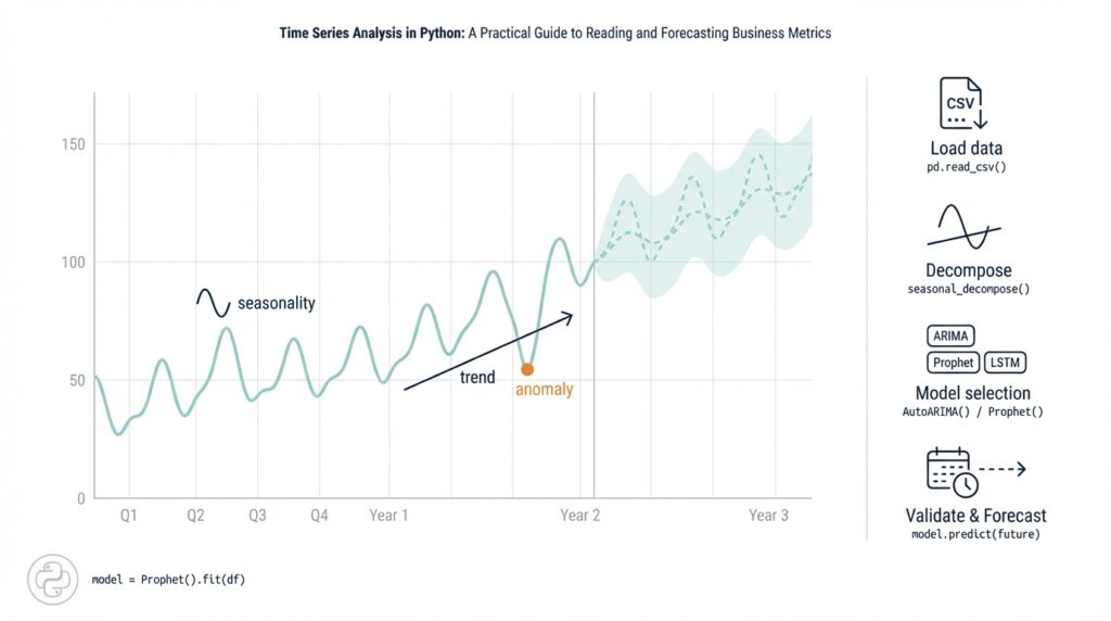
Building on this foundation, the fastest way to gain actionable insight is visual exploration that makes the trend and seasonality explicit in your time series. Start by plotting the full series with a robust smoother and a decomposed seasonal component so you immediately see long-run drift, changing amplitude, and recurring cycles. Visual diagnostics should be the first filter before any heavy preprocessing: they tell you whether seasonality is stable, multiplicative, or drifting, and they guide choices like log transforms, seasonal differencing, or time-varying models.
Decomposition is the workhorse for separating trend from repeated patterns, and STL (Seasonal-Trend-Loess) is often a better first choice than classical additive decomposition because it handles non-stationary seasonality and outliers. Use STL to extract trend, seasonal, and residual components and inspect them side-by-side; set the period to your expected cycle (7 for weekly, 365 for daily-yearly) and enable robust=True when spikes or outages exist. For example:
from statsmodels.tsa.seasonal import STL
res = STL(df['metric'], period=7, robust=True).fit()
res.trend.plot(); res.seasonal.plot()
Comparative seasonal plots make repeating patterns easy to interpret for business stakeholders. Create seasonal subseries (group by month or weekday and overlay years) to reveal shifts in timing or amplitude, and build an hour-of-week heatmap for high-frequency metrics like traffic or CPU load so you can see where the daily-weekly interaction concentrates. A concise pivot + heatmap looks like:
pivot = df['metric'].groupby([df.index.isocalendar().week, df.index.weekday]).mean().unstack()
sns.heatmap(pivot, cmap='magma')
These views reveal common practical issues: a weekday peak that drifts into weekends, a holiday spike that repeats each year, or a seasonal amplitude that grows over time. Overlaying year-on-year lines (aligning calendars) is particularly effective for product teams who ask, “Is this month’s growth seasonal or structural?” — the visual answer often beats a p-value.
When you don’t know the dominant period, use autocorrelation and spectral methods to detect periodicities before you assume them. Plot the ACF/PACF to identify candidate lags for seasonal difference or features, and compute a periodogram to find dominant frequencies when multiple seasonalities exist (daily + weekly + yearly). Short code sketches:
from statsmodels.graphics.tsaplots import plot_acf
plot_acf(df['metric'].dropna(), lags=168)

from scipy.signal import periodogram
f, Pxx = periodogram(df['metric'].fillna(0))
dominant = 1 / f[1:][Pxx[1:].argmax()]
Interactivity accelerates hypothesis testing: use Plotly or Altair to pan, zoom, and toggle decomposition layers so you can instantly check whether a suspected calendar event caused a spike. Annotate known campaigns, deployments, or holidays and compare the seasonal component before and after the event to detect structural breaks. Also decide visually whether seasonality is multiplicative (variance scales with level) or additive — if amplitude scales, a log transform will linearize effects and simplify modeling.
The practical payoff of careful visualization is clearer modeling decisions: stable seasonality suggests fixed seasonal terms (Fourier features or SARIMA), drifting amplitude points to STL-based adjustments or state-space models, and multiple overlapping cycles push us toward TBATS, Prophet, or neural architectures that accept multiple seasonal periods. How do you choose the right visualization to surface business-season patterns? Use these plots iteratively: decompose, inspect ACF/periodogram, visualize subseries and heatmaps, then convert the insights into concrete features or model structures for forecasting. Transitioning from visual insight to feature engineering will be our next concrete step.
Resample, clean, and impute
Building on this foundation, the first practical preprocessing step is to resample, clean, and impute your time series so downstream models see a regular, trustworthy signal. You should front-load this work because resampling and imputation change both the statistical properties and the business meaning of the metric: counts, rates, and ratios require different aggregation and filling rules. Assume UTC-indexed, frequency-consistent data from the previous step and decide a target cadence (hourly, daily, weekly) that preserves business semantics before you change anything. How do you pick that cadence and the right aggregation? We’ll walk through the choices and show concrete patterns you can apply immediately.
Start by choosing a target frequency and an aggregation semantics that preserve meaning. For downsampling event logs to a daily business metric, use df.resample('D').sum() for counts and df.resample('D').mean() for rates; avoid asfreq when raw timestamps are irregular unless you explicitly want gaps preserved. Upsampling (e.g., daily→hourly) should be paired with a well-defined fill strategy because naive expansion creates artificial continuity; use df.resample('H').ffill(limit=2) only for short gaps where propagation is defensible. If your series contains mixed granularities, choose the coarsest frequency that retains signal for forecasting and collapse higher-resolution rows with aggregation functions that reflect business logic.
Cleaning the series is about eliminating structural errors and annotating anomalies rather than aggressive smoothing that erases signal. Remove duplicate timestamps with df = df[~df.index.duplicated(keep='last')] and align timezone-aware indices so joins don’t produce phantom gaps. Detect outliers with a robust measure (IQR or rolling MAD) and decide: cap, mask, or leave them depending on whether they represent real business events. For example, use q_low, q_high = metric.quantile([0.01, 0.99]) then df['metric'] = df['metric'].clip(q_low, q_high) to limit extreme sensors errors while preserving legitimate spikes for forecasting.
Imputation should be deliberate: choose a method that matches the causal mechanism of missingness and the metric type. Simple imputation like df['metric'].interpolate(method='time') or df.fillna(method='ffill', limit=3) works well for short, random gaps in a stationary series, while seasonal interpolation (fit over the same weekday/hour across past cycles) suits recurring patterns. For long outages or post-deployment gaps consider model-based imputation (state-space models, Prophet-style trend+seasonality, or KNN for multivariate gaps) and always create an is_imputed indicator so models can learn different behavior on imputed values. Ask yourself: will this fill introduce lookahead bias? Never use future data when imputing training or validation windows.
Apply a concrete business example to make this concrete: suppose you have hourly web traffic logs with intermittent missing minutes and occasional deployment-induced outages. Resample to hourly using df = df.resample('H').sum() to preserve counts, drop or merge duplicated hours, and forward-fill short (≤15 minute equivalent) gaps with ffill(limit=1). For multi-hour outages, interpolate using the same hour-of-week seasonal average or flag the entire outage and impute with a seasonal model trained on comparable days. Also add df['missing_rate'] = df['metric'].isna().astype(int).rolling(24).mean() so your model knows when data quality was poor.
Validate every imputation choice with backtesting and holdout periods to quantify forecast sensitivity to filling decisions. Use rolling-window cross-validation where you apply the exact imputation pipeline inside each fold to avoid leakage; compare metrics with and without imputed segments masked or flagged. Visually compare original, cleaned, and imputed series with overlays of is_imputed to confirm you didn’t smooth away real campaign spikes or introduce artificial seasonality. This empirical validation is the only way to know whether a chosen imputation strategy helps or harms forecasting performance.
After you’ve resampled, cleaned, and imputed, preserve provenance: keep original timestamps, a missingness indicator, and a concise log of transformations so features and models can be audited. These artifacts let you reason about model errors later and allow feature-engineering steps—lags, rolling windows, Fourier terms—to be applied consistently. In the next section we’ll use these cleaned series to construct lagged features and seasonal components that improve predictive accuracy while avoiding common pitfalls introduced during preprocessing.
Test stationarity and decompose
Building on this foundation of visual inspection and STL-based decomposition, the next practical step is to test whether the series is stationary and, if not, determine how to remove trend and seasonality so models behave predictably. Stationarity—roughly, constant mean and variance over time—is a prerequisite for many linear forecasting models because non-stationary data produce spurious correlations and unstable parameter estimates. We’ll show a repeatable workflow: run unit-root and stationarity tests, inspect ACF/PACF of raw and differenced series, apply variance-stabilizing transforms, and re-check stationarity on residuals after decomposition.
Start with two complementary statistical checks: the Augmented Dickey-Fuller (ADF) for a unit root and the KPSS test for level stationarity. The ADF’s null hypothesis is that a unit root exists (non-stationary), while KPSS has the reverse null (stationary), so using both reduces false conclusions. How do you interpret mixed signals? If ADF fails to reject and KPSS rejects, you have strong evidence of non-stationarity and should consider differencing or detrending; if both indicate stationarity, you can proceed to modeling without differencing.
In code, a minimal reproducible check looks like this (using statsmodels):
from statsmodels.tsa.stattools import adfuller, kpss
x = df['metric'].dropna()
adf_result = adfuller(x)
kpss_result = kpss(x, regression='c')
print('ADF p-value:', adf_result[1])
print('KPSS p-value:', kpss_result[1])
When tests show non-stationarity, choose the simplest corrective action that preserves business meaning. For a deterministic trend, remove it by detrending (OLS or a rolling/LOESS smoother) or take first differences to remove a stochastic trend. For recurring patterns, apply seasonal differencing with the known period (e.g., diff(periods=7) for weekly seasonality on daily data). Always re-run ADF/KPSS after each transformation to confirm stationarity rather than assuming differencing helped.
Variance that grows with level demands a variance-stabilizing transform before differencing; the log transform or a Box–Cox transform is the usual choice. Apply log for positive, multiplicative seasonality and use Box–Cox when a parametric lambda gives a better stabilization. For example:
from scipy.stats import boxcox
y, lam = boxcox(df['metric'].dropna() + 1e-6)
# then test y for stationarity and difference as needed
Decomposition remains central: after STL or classical decomposition, test stationarity on the residual (remainder) component rather than the raw series. If the residual is stationary, your trend+seasonal model successfully captured non-stationary components and you can model the remainder with ARMA-like structures. If residuals still show autocorrelation or non-constant variance, iterate on decomposition settings: adjust STL’s seasonal window, switch robust fitting on, or try multiplicative decomposition when amplitude scales with level.
Practical diagnostics complete the loop: inspect ACF/PACF plots of both the transformed series and residuals to choose differencing orders and AR/MA lags, and run Ljung–Box tests for remaining serial correlation. For multiple overlapping seasonalities (hourly + weekly + yearly) a single seasonal differencing may be insufficient; consider Fourier terms, TBATS-like approaches, or state-space seasonal components instead of aggressive differencing that destroys long-run signal. Also guard against structural breaks: perform rolling ADF/KPSS or segmented decomposition around known events (deploys, product launches) and treat break periods differently in modeling or validation.
Taking these steps ensures the series you feed into forecasting algorithms has predictable statistical behavior and clear provenance for each transform. After you’ve confirmed stationarity on residuals and recorded transforms (log/Box–Cox, differencing orders, seasonal period), we can convert those insights into lagged features, Fourier terms, or state-space specifications for the models in the next section.
Engineer lags and features
Building on this foundation, the most important lever you have for predictable forecasts is disciplined lag feature construction—because good lag features encode the signal history your model actually needs. Time series model performance hinges less on exotic algorithms and more on which past values and aggregates you expose to the learner, so we should treat lag selection as a design problem informed by both diagnostics and business logic. How do you choose lags that actually improve forecast accuracy? Start with autocorrelation diagnostics and concrete business cycles, then iterate with robust validation.
Use statistical diagnostics to narrow candidate lag windows before you generate hundreds of columns. Plot the ACF/PACF from the previous section to expose strong short-term and seasonal autocorrelations, but overlay domain-driven lags too: include 1, 7, 14, 28 for daily metrics with weekly/monthly effects, or 1, 24, 168 for hourly series with diurnal and weekly cycles. Combine these diagnostics with event knowledge—campaigns, payroll dates, releases—to add targeted lagged indicators rather than broad brute-force expansion; this keeps feature engineering tractable and interpretable.
Implement lagged and rolling features as reproducible transforms in your preprocessing pipeline rather than ad-hoc DataFrame edits. Use pandas shifts and window ops inside a function you can apply in each CV fold to avoid leakage:
def make_lags(df, col):
    df[f'{col}_lag1'] = df[col].shift(1)
    df[f'{col}_ma7'] = df[col].rolling(7).mean().shift(1)
    df[f'{col}_std14'] = df[col].rolling(14).std().shift(1)
    return df
Always shift rolling aggregates so the model never sees future information. We recommend encapsulating these operations in a transformer (sklearn or custom) and calling it inside the same time-based split used for backtesting so your experiments mirror production behavior.
Beyond raw lags, engineer derived signals that capture directionality, scale, and seasonality interactions. Create difference lags (x_t – x_{t-1}), percent-change features, normalized lags (divide a lag by a longer-term rolling mean), and interaction terms with calendar flags (hour-of-week × lag). For example:
df['lag24_norm'] = df['metric'].shift(24) / df['metric'].rolling(168).mean().shift(24)
These normalized and interaction features often help models generalize across non-stationary regimes where level and amplitude change.
Be deliberate about selection and regularization: many lagged features are highly collinear and can destabilize linear models. Apply L1/L2 regularization, tree-based feature importance checks, or dimensionality reduction (PCA on lag blocks) to prune redundant columns. Use permutation importance or SHAP in validation folds to confirm that retained lags add incremental predictive value rather than fitting transient noise. Also maintain an is_imputed flag and any provenance columns so the model can learn when values were reconstructed—this is essential when you used the imputation strategies described earlier.
Finally, design for operational scale: generating dozens of lag and rolling features multiplies storage and compute. Compute offline feature tables for training, and implement streaming or incremental aggregations for online serving to avoid expensive window scans at prediction time. If you rely on a feature store or cached tables, version the transformations so you can reproduce training features in production and during backtests.
With a concise set of well-justified lag features and derived aggregates, your models will have the historical context they need without overfitting to spurious autocorrelations. Next, we’ll take these engineered predictors into model selection and cross-validation, where we can measure which lags carry predictive power across realistic holdout windows.
Build and evaluate forecasting models
Building on the preprocessing and feature engineering work we just covered, the next practical step is to actually build and evaluate forecasting models that will drive decisions. Start by treating model choice as a hypothesis about the data-generating process: are you modeling a stable linear process, a state-space trend with changing seasonality, or nonlinear interactions driven by external covariates? Framing model selection this way keeps us focused on business value rather than model novelty and gets you to measurable improvements in forecast accuracy faster. If you think multiplicative seasonality dominates, try variance-stabilizing transforms before fitting any candidate model.
Choose candidate families pragmatically: simple exponential smoothing and state-space (ETS) models for strong, smooth trends; ARIMA or SARIMAX when autoregressive structure explains short-term persistence; gradient-boosted trees (e.g., XGBoost/LightGBM) for rich lag/feature sets; and lightweight neural nets or temporal convolution models when you have long histories and many covariates. Each class has trade-offs: statistical models give interpretable components and calibrated intervals, while machine learning models often excel at capturing nonlinear interactions but need careful feature pipelines to avoid leakage. We recommend starting with a simple statistical baseline and adding complexity only when it reduces out-of-sample error and preserves interpretability for stakeholders.
How do you structure cross-validation for time series so that your evaluation reflects production behavior? Use rolling-origin (also called time series split) validation where each fold trains on an earlier contiguous block and tests on a later holdout, and ensure that the full imputation, scaling, and lag generation pipeline is executed inside each fold. Prefer an expanding-window when your goal is to mimic continuous retraining (train on t0..tN then t0..tN+k) and a sliding-window when stationarity is plausible and you want to limit model memory. Implementing cross-validation correctly prevents lookahead bias and produces realistic estimates of forecasting models’ out-of-sample performance.
Pick evaluation metrics that align to business impact rather than convenience. Use MAE when absolute errors map directly to costs, RMSE when large errors are disproportionately harmful, and scale-free measures like MAPE or SMAPE when you need comparability across entities with different scales. For revenue or conversion-rate forecasts where downside risk matters, optimize and report quantile losses or pinball loss to reflect asymmetric business tolerances. Track both point-forecast metrics and probabilistic coverage (e.g., 80–95% prediction interval coverage) because well-calibrated intervals are crucial for capacity planning and risk-aware decisions.
Make model selection reproducible by embedding hyperparameter search into the time-aware CV loop: grid or random search, or Bayesian tuning, but always evaluate candidates using the same rolling-origin splits. Pipeline your preprocessing (imputation, lag creation, scaling, categorical encodings) so that every trial applies identical transforms; otherwise hyperparameter gains will be artifacts of inconsistent pipelines. After selecting a model, run a final backtest that simulates deployment (walk-forward evaluation) yielding a time-ordered error series that you can audit for structural breaks and seasonal miscalibration.
Diagnostics and calibration matter as much as point accuracy. Inspect residual autocorrelation, heteroskedasticity, and error drift over calendar time or by campaign segments; persistent patterns indicate missing features or regime shifts rather than model failure. For probabilistic forecasts, evaluate sharpness and calibration: narrow intervals are desirable only when they maintain nominal coverage. If prediction intervals under-cover during high-variance periods, add heteroskedastic components (state-space variance models, quantile regression forests) or use ensemble techniques to blend diverse model assumptions.
Taking this concept further, operationalize evaluation: automate nightly backtests, store fold-level metrics, and version both feature code and model artifacts so you can reproduce any forecast. When you move to production, implement a simple monitoring dashboard that tracks forecast accuracy, interval coverage, and drift in input features so we can schedule retraining before accuracy degrades materially. This disciplined feedback loop closes the gap between time series forecasting experiments and forecasts you can rely on for business decisions.