Why Tokens and Embeddings Matter
Building on this foundation, understanding tokens and embeddings is the practical difference between a model that feels useful and one that feels random. Tokens and embeddings are the two plumbing layers you will touch every time you design prompts, optimize cost, or implement retrieval-augmented workflows for LLMs; they directly shape latency, accuracy, and developer ergonomics. How do you reason about token budgets, semantic search quality, and the trade-offs between on-the-fly context vs. vector retrieval? We’ll make those trade-offs concrete so you can design systems with predictable behavior.
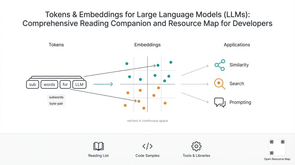
Start with tokens because they drive the input/output economics and the model’s effective memory. A token is a unit of text produced by the tokenizer (subword pieces, not necessarily words), and how text gets split determines prompt length, truncation behavior, and billing. When you concatenate user history, documents, and system instructions, you’re adding tokens to the same billable context window; that means long documents can force truncation or expensive long-context models. In practice, measure token counts early in development with the same tokenizer you’ll use in production and treat token budgeting as an operational constraint, not an afterthought.
Embeddings convert text into dense numerical vectors that capture semantic relationships, and they’re what enable semantic search, clustering, and similarity-based retrieval. Think of embeddings as coordinates in a high-dimensional semantic space: semantically similar sentences end up nearby in vector distance (cosine similarity is a common metric). You’ll use embeddings to index knowledge bases, build nearest-neighbor retrieval, or group documents for summarization. This separation—cheap vector lookup for broad relevance and expensive LLM generation for fluent responses—is the core performance pattern for scalable conversational systems.
Here’s a minimal pattern you’ll implement repeatedly: encode → index → retrieve → synthesize. In Python-like pseudocode it looks like:
texts = [doc1, doc2, doc3]
vectors = embedder.encode(texts, batch_size=32)
vector_store.upsert(ids, vectors, metadata)
results = vector_store.search(query_vector, top_k=5)
prompt = assemble_prompt(results, user_query)
response = llm.generate(prompt)
This pipeline exposes two design knobs: how you chunk source text before embedding, and how many retrieved chunks you stitch into the prompt. Both knobs interact with token limits and relevance.
The interplay between tokenization and embeddings is where design mistakes surface. If you embed huge documents without chunking, you lose locality—retrieval returns a long blob that consumes tokens and dilutes relevance. If you chunk too small, you fragment context and increase false positives during similarity search. A pragmatic compromise is semantic-aware chunking (split at paragraph/section boundaries, preserving meaning) with windowed overlap so retrieved passages maintain continuity. Also account for embedding dimensionality and index footprint: larger embedding vectors improve nuance but increase storage and approximate nearest neighbor (ANN) search cost.
Finally, this affects operational decisions: tokens determine per-request cost and model choice; embeddings determine storage, index latency, and retrieval precision. When performance matters, batch embedding requests to reduce overhead, precompute embeddings for stable documents, and instrument end-to-end latency from query to LLM response including retrieval time. We often measure relevance with human-in-the-loop evaluation and A/B test prompt assembly strategies to balance precision vs. prompt length.
Taking this concept further, treat tokens and embeddings as co-evolving system primitives rather than isolated tools. When you design a knowledge retrieval flow, decide first how you’ll represent content (chunk size, metadata), then how you’ll budget tokens for prompt composition, and finally which embedding/index combo meets your latency and precision targets. That sequence—represent, budget, select—keeps decisions predictable and gives you levers to tune as usage scales.
Tokenization Algorithms and Tradeoffs
Building on this foundation, the practical choice of how you split text shapes cost, latency, and semantic fidelity more than most architecture decisions. Start by remembering that tokenization is not an implementation detail: it defines the atomic units your model and embeddings operate on, and that directly affects your token budget and the semantic granularity of retrieval. We’ll walk through common algorithms, show where they fail in real systems, and give rules of thumb you can apply when you must choose between vocabulary size, robustness, and speed.
The dominant families of tokenizers are byte-pair style approaches (BPE and byte-level BPE), WordPiece, and unigram (a.k.a. SentencePiece unigram). Each takes a different stance on the core trade-off: larger vocabularies keep frequent whole words as single tokens but increase model embedding tables and OOV complexity, while smaller vocabularies produce many subword pieces which increase token counts and sometimes hurt prompt readability. BPE merges frequent symbol pairs greedily, WordPiece uses a likelihood hinge for merges, and unigram treats tokenization as selecting the most probable segmentation under a language model. These algorithmic choices manifest in predictable behaviors: BPE variants are fast and compact for English-like corpora, unigram can be more robust for morphologically rich languages, and byte-level BPE handles arbitrary binary/emoji inputs without requiring normalization.
How do you choose between BPE, WordPiece, and unigram tokenizers for your data? The decision hinges on three practical axes: token budget, noise robustness, and vocabulary maintenance. If you’re optimizing for minimal token count and your corpus is stable English text, a moderate-size BPE vocabulary (30k–50k tokens) often yields the best cost/performance trade-off. If you must support many languages, messy user input, or arbitrary file formats, prefer byte-level tokenizers or larger unigram models because they avoid brittle normalization and reduce unknown-token failure modes that break downstream embedding quality.
A concrete example makes the trade-offs tangible. Suppose a 1,000-word technical doc contains many identifiers, code snippets, and URLs. With a word-level view you might see ~1,000 tokens, but with a subword tokenizer those identifiers break into dozens of pieces, inflating prompt length and the embedding vector budget. In Python pseudo-pattern using a Hugging Face style tokenizer, measure early:
tokens = tokenizer.encode(doc)
print(len(tokens))  # use this count when budgeting token_budget
emb = embedder.encode(doc)
Always measure counts with the exact tokenizer used by both your LLM and your embedder; mismatched tokenizers produce inconsistent token counts and can degrade embeddings because the same semantic unit maps to different subword sequences.
There are operational trade-offs beyond raw counts. Larger vocabularies increase model parameter size and embedding table memory, which raises inference cost and storage for precomputed embeddings. Smaller subword pieces increase ANN index size (more vectors or more fragments per document) and can raise false positives during retrieval because semantic signals get fragmented. Moreover, deterministic byte-level tokenizers simplify caching and deduplication, while language-aware tokenizers can improve semantic embedding quality for natural text but complicate normalization rules for code and log data.
Given these trade-offs, apply simple rules of thumb: measure token counts and retrieval precision on representative inputs; prefer byte-level or unigram when input is heterogeneous; tune vocabulary size when you control the training pipeline; and always align tokenizer choice between embedding generation and LLM prompting. Taking these steps reduces surprises in token budgeting and ensures embeddings remain meaningful as you scale retrieval-augmented generation systems.
Vocabulary, Token IDs, Mappings
Building on the tokenizer trade-offs we’ve already covered, understanding how the model’s vocabulary, token IDs, and mappings work in practice is where many engineering bugs begin. The vocabulary is the canonical list of tokens the tokenizer and model agree on; token IDs are the integer indices the model uses at inference time; mappings are the bidirectional functions that convert text ↔ tokens ↔ IDs. If you treat these artifacts as implementation details, you’ll run into silent failures in caching, embedding lookup, and fine-tuning pipelines.
Start by inspecting the concrete data structures your tooling exposes. A tokenizer usually exposes a vocabulary table (string → id) and APIs to convert back (id → string). This table is not cosmetic: the embedding matrix rows are indexed by the token ID, so a mismatch between tokenizer vocabulary and model weights means the wrong embedding is pulled for a token. In practice, always call the tokenizer’s vocabulary inspection routines during initialization so you can assert consistency: mismatched sizes or missing special tokens should fail fast rather than manifest as subtle quality regressions.
Here’s a minimal example of the common pattern you’ll use when verifying alignment in Python-like libraries:
vocab = tokenizer.get_vocab()           # dict: token -> id
tokens = tokenizer.encode(text)
ids = tokenizer.convert_tokens_to_ids(tokens)
reconstructed = tokenizer.convert_ids_to_tokens(ids)
assert tokenizer.decode(ids) == tokenizer.decode(tokens)
This small check catches many accidental remappings. Keep a versioned copy of the vocabulary file with your model artifacts and assert the vocabulary size matches the embedding matrix shape during startup. When you extend a vocabulary (adding domain-specific tokens), remember that new token IDs shift the index space unless you append IDs and update the model embedding matrix correspondingly.
Practical systems often break when tokenizers change mid-flight. Suppose you precompute embeddings for documents with Tokenizer A and later serve queries using Tokenizer B—the same word pieces can map to different token IDs or split differently, yielding embeddings that no longer align in vector space. How do you avoid that? We keep a tokenizer version or fingerprint in metadata with every stored embedding, and reject or re-embed documents whose tokenizer fingerprint differs from the current serving tokenizer. Alternatively, maintain a stable, canonical vocabulary and grow it only in append-only fashion, remapping and padding the embedding matrix when you introduce new IDs.
Special and reserved tokens deserve particular attention because they affect decoding, prompt assembly, and retrieval heuristics. Tokens like or occupy fixed IDs and should be present in both tokenizer and model; missing or shifted reserved IDs will corrupt prompt templates and truncation logic. When assembling prompts from retrieved chunks, prefer converting back to text with tokenizer.decode(ids, skip_special_tokens=True) so you don’t accidentally inject control tokens into user-visible text; conversely, include special tokens intentionally when you rely on them for instruction boundaries or segment embeddings.
Finally, adopt a few engineering patterns that scale: store tokenizer name+SHA alongside embeddings and model checkpoints; assert vocabulary size == embedding_matrix.shape[0] at load time; log token ID histograms for production requests to detect distributional shifts; and, when you must change tokenizers, run a small A/B of re-embedded documents to measure retrieval precision before rolling out. By treating the vocabulary, token IDs, and mappings as first-class, versioned artifacts rather than ephemeral internals, we make embedding-based search and prompt composition predictable and debuggable as systems scale.
Embedding Types and Representations
Building on this foundation, the choices you make about representation determine how well retrieval and downstream LLM synthesis work in real systems. Embeddings are not a single, monolithic thing — they come in flavors that trade off precision, speed, and storage. Front-load this decision: pick an embedding type that matches your use case (retrieval, classification, token-level alignment) because the downstream index, ANN settings, and prompt budget will follow from that choice.
A first major axis is static versus contextual representations. Static embeddings (word2vec, GloVe) map a token to a fixed vector regardless of sentence context; contextual embeddings (transformer-based models like BERT-derived encoders or sentence-transformers) produce vectors that reflect surrounding words and sentence intent. For document-level semantic search and paraphrase matching, contextual sentence embeddings capture nuance and disambiguation that static vectors cannot, whereas static vectors remain useful for lightweight, cache-friendly features or when you need predictable, token-level lexical signals.
Another crucial distinction is sparse versus dense representations. Sparse vectors (TF-IDF, BM25, or learned sparse transformers) represent text as high-dimensional but mostly-zero vectors that excel on lexical matching and are interpretable; dense vector embeddings are low-dimensional continuous vectors learned to place semantically similar text nearby. Which should you use? If exact lexical overlap and explainability matter, choose sparse; if paraphrase robustness and semantic recall matter, choose dense semantic vectors and tune your ANN index accordingly.
How you convert token outputs into a single representation matters as much as which model you choose. Pooling strategies—mean pooling across token vectors, using a CLS token, or attention-pooling—produce different inductive biases: mean pooling often smooths noise across long passages, CLS captures a model-trained summary vector, and attention-pooling can emphasize salient spans. In practice, implement and compare a few approaches; for example, with a sentence-transformer-like encoder you might use mean pooling but apply L2 normalization afterward:
tokens = encoder.tokenize(text)
hidden = encoder.forward(tokens)       # [seq_len, dim]
vec = hidden.mean(axis=0)              # mean-pool
vec = vec / np.linalg.norm(vec)        # L2 normalize for cosine distance
Multilingual and multimodal representations are increasingly common in production. Multilingual embeddings map different languages into a shared semantic space so cross-lingual retrieval works without translation; multimodal embeddings jointly encode text, images, or audio so you can retrieve images by caption or vice versa. We often build composite representations by concatenating a dense semantic vector with a sparse lexical fingerprint (TF-IDF or hashed n-grams) to get the best of both worlds: semantic recall plus lexical precision. Also consider operational transforms like dimensionality reduction (PCA) or quantization (int8, product quantization) when index size and ANN latency are primary constraints.
Representation hygiene is practical, not academic. Normalize vectors when you’ll use cosine similarity; preserve magnitude when dot product and vector norms encode confidence. When you precompute embeddings, store the embedder version, pooling method, dimensionality, and normalization flag in metadata so you never mix incompatible vectors at query time. How do you validate a choice? Measure recall@k and mean reciprocal rank on representative queries, profile index memory and search latency, and run small A/B tests that vary embedding dimensionality and pooling.
Taken together, these representation choices change how the rest of your system behaves: index size, ANN configuration, retrieval precision, and prompt budget. As we move to implementation patterns, we’ll use these distinctions to pick chunking strategies, index types, and evaluation metrics so you can iterate from an informed baseline rather than guesswork.
Similarity Metrics and Evaluation
Building on the embedding and tokenization groundwork, measuring similarity is the practical lever that turns vectors into reliable retrieval signals—cosine similarity and embedding evaluation are where you separate useful recall from noise in semantic search. We start by recognizing that not all distance functions behave the same across embedder types; cosine similarity is stable when vectors are L2-normalized, while dot product can encode magnitude-based confidence for some models. How do you choose the right metric for retrieval in practice? The right choice depends on your embedder’s training objective, whether you preserve vector norms, and the downstream goal (ranking vs. binary match).
A compact taxonomy helps: cosine similarity, dot product, and Euclidean (L2) distance are the usual suspects. Cosine similarity measures angle and is robust when you want scale invariance—normalize vectors and use cosine for paraphrase and semantic matching. Dot product favors vectors with larger norms and can be useful when the embedder encodes confidence in magnitude; use it when your model was trained with inner-product objectives or when you rely on unnormalized logits. Euclidean distance is rarer for sentence embeddings but can expose locality structure when you’ve applied dimensionality reduction or quantization; always validate with empirical tests rather than assumptions.
Ranking and retrieval evaluation needs targeted metrics: recall@k, precision@k, mean reciprocal rank (MRR), and nDCG each answer different product questions. Recall@k tells you whether relevant documents appear in the candidates you’ll send to the LLM; precision@k measures noise among those candidates and directly affects prompt quality and token budget. MRR emphasizes getting the very best result at top rank, which matters for single-answer flows, while nDCG accounts for graded relevance and diminishing utility down the rank list—useful when passages have different usefulness scores. Choose metrics that mirror your user experience: if you assemble three retrieved chunks into a prompt, optimize recall@3 and precision@3 alongside a human relevance score.
A short Python-like example clarifies the pattern: compute cosine scores, sort, then measure recall@k on labeled queries.
q_vec = embed(query)
docs = embedder.encode(batch_docs)
scores = (docs @ q_vec) / (np.linalg.norm(docs, axis=1)*np.linalg.norm(q_vec))  # cosine
ranked = np.argsort(-scores)
relevant_in_top_k = any(labelled[ranked[:k]])
recall_at_k = sum(relevant_in_top_k)/len(queries)
This snippet shows a pipeline you’ll run during offline evaluation; normalize consistently, compute metrics over realistic query sets, and log per-query failures to drive hard-negative mining.
Dataset design and negative sampling often determine how trustworthy your evaluation is. Use in-domain queries and realistic negatives: random negatives overestimate performance while hard negatives (semantically similar but irrelevant) simulate production confusion the model will face. Create temporal splits to surface embedding drift—documents added after your embeddings were precomputed often reveal versioning problems we discussed earlier—and include synthetic paraphrases to test robustness to rephrasing. Labeling strategy matters too: graded labels allow nDCG-style evaluation, while binary labels simplify monitoring but can hide nuance.
Production monitoring and online evaluation close the loop between offline metrics and user impact. Run small A/B experiments that vary retrieval metric (cosine vs dot), ANN parameters, or top-k sizes and measure downstream metrics like click-through, resolution rate, and LLM hallucination incidents. Instrument index-level signals: average similarity score, proportion of results below an operational threshold, ANN recall loss due to quantization, and latency tail metrics. When you convert similarity to a binary decision, calibrate thresholds on held-out traffic and retrain thresholds periodically as embeddings and tokenization change.
Finally, make evaluation an iterative workflow: log failures, mine hard negatives, re-evaluate with both offline scores and targeted human judgments, and then run short online rollouts to validate product impact. Maintain metadata with embedder version, pooling method, and tokenizer fingerprint for every stored vector so you can roll back or re-embed consistently. By treating similarity measurement and embedding evaluation as continuous engineering tasks—not one-time experiments—you keep retrieval predictable, improve prompt quality, and reduce surprise regressions as your system scales.
Practical Tools, Workflows, Resources
Building on this foundation, the difference between a research diagram and a production system comes down to the tools and workflows you choose to operationalize tokens and embeddings. You already know tokens drive cost and context, and embeddings power semantic search and retrieval—front-load those words because they should appear in your tooling choices and observability dashboards within the first days of development. If you don’t bake in token accounting and embedder versioning from day one, you’ll rapidly encounter subtle mismatches that break retrieval quality and inflate bills.
Start by choosing the pragmatic categories of tooling we’ll rely on: a tokenizer and tokenizer validator, an embedder (encoder) with clear versioning, a vector store with ANN capabilities, and the orchestration code that implements encode → index → retrieve → synthesize. Each component has operational knobs: tokenizer normalization affects token counts, the embedder’s dimensionality affects index size, and ANN parameters affect tail latency. We recommend thinking of these as interchangeable modules you can swap and benchmark rather than lock into a single vendor or library.
For everyday workflows, implement the encode → index → retrieve → synthesize pipeline as a reproducible CI-tested job. Write small, testable scripts that batch-embed new documents, attach metadata including tokenizer SHA and embedder version, upsert vectors into a vector store, and expose a retrieval API that returns both vectors and tokenized lengths for prompt budgeting. A minimal pseudocode example clarifies the pattern:
vecs = embedder.encode(docs, batch_size=64)
for id, vec, md in zip(ids, vecs, metas):
    vector_store.upsert(id, vec, metadata=md)
candidates = vector_store.search(query_vec, top_k=5)
prompt = assemble_prompt(candidates, query, token_budget=2048)
response = llm.generate(prompt)
Chunking and batching are where many systems win or fail in practice. When you chunk, preserve semantic boundaries—split at paragraphs, headings, or code blocks—and use a modest overlap window so retrieved passages maintain continuity; when you batch embeds, amortize per-request overhead to reduce latency and cost. Always compute token counts with the same tokenizer you use for prompt assembly and store those counts alongside vectors so you can make deterministic prompt-construction decisions at request time. As we discussed earlier, tokenizer alignment between precomputed embeddings and runtime prompts is non-negotiable.
How do you choose the right vector store or ANN index for low-latency retrieval? Evaluate based on three operational axes: search latency (p95/p99), index memory footprint, and query recall loss introduced by quantization or approximations. HNSW-style indices give excellent recall and low-latency at the cost of memory; IVF/PQ or product-quantized indices reduce storage but need careful calibration to avoid recall degradation. Also test practical features: persistent metadata filtering, real-time upserts, distributed replication, and built-in metrics—these determine whether a vector store fits your production SLAs.
Monitoring and lifecycle workflows keep embeddings trustworthy over time. Instrument token counts per request, average cosine similarity of top results, recall@k on a small held-out labeled set, and end-to-end latency from query to LLM response. Version every stored embedding with embedder_id, tokenizer_fingerprint, pooling_method, and normalization_flag; when the embedder or tokenizer changes, run an automated re-embed pipeline or mark vectors for lazy re-embedding and measure retrieval regressions with hard-negative mining. We use small A/B experiments and shadow traffic to validate re-embedding before rolling changes wide.
For practical resources, start with stable libraries and a shortlist of vector stores so you can prototype fast and replace pieces cleanly: tokenizer and embedder tooling from widely used ecosystems, an ANN library for local experiments (FAISS or an HNSW implementation), and a managed or open-source vector store when you need scale (choose one that supports metadata filters and real-time upserts). Keep a canonical test corpus and a query suite that represent real user intent so your semantic search metrics reflect production behavior rather than synthetic benchmarks.
Taking these practices together, we turn conceptual decisions about tokens and embeddings into repeatable engineering artifacts: versioned tokenizers, metadata-rich embeddings, measured ANN choices, and observability dashboards that track recall and cost. In the next section we’ll apply these implementation choices to chunking strategies and prompt assembly heuristics so you can iterate from a measured baseline rather than guesses.