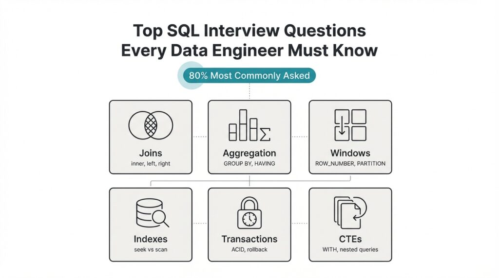
Core SQL Concepts
Building on this foundation, mastering a few fundamental relational concepts will get you through most SQL interview questions and make you a stronger data engineer. Start by treating the relational model as the contract between your data and queries: tables represent entities, columns represent attributes, and foreign keys express relationships. Understanding normalization levels (1NF–3NF) helps you decide when to denormalize for performance, and knowing when to trade storage for faster reads is a practical decision you’ll justify during interviews and on the job.
The next core idea is how joins express relationships at query time. INNER, LEFT, RIGHT, and FULL joins let you control whether unmatched rows survive the match; each choice has semantic and performance implications. For example, when reconciling orders with optional refunds use a LEFT JOIN to preserve orders that lack refunds; if you need only matched pairs, an INNER JOIN is clearer and often faster. Watch out for join explosion — joining large tables without selective predicates multiplies rows and costs you CPU and I/O.
Aggregations and grouping are where raw data becomes insight, so understand GROUP BY, aggregate functions, and HAVING as distinct tools. GROUP BY collapses rows by key, aggregates compute summaries, and HAVING filters after aggregation — misplacing predicates between WHERE and HAVING is a common interview trap. For example, WHERE event_time >= '2025-01-01' reduces input rows before aggregation, while HAVING count(*) > 1 filters groups after aggregation; choose the right one to reduce work and get correct results.
Window functions are a leap beyond classic aggregation because they let you compute row-level results that reference related rows. Use ROW_NUMBER() for deterministic deduplication, RANK()/DENSE_RANK() for ties, and SUM(...) OVER (PARTITION BY ... ORDER BY ...) for running totals and sliding-window analytics. How do you pick between aggregation and window functions? Use aggregation when you want one row per group; prefer window functions when you need both detail rows and group-level context in the same result set.
Indexes and execution plans determine whether your SQL performs at production scale; you must read a query plan and reason about cost. Favor B-tree indexes for range and equality predicates, and consider bitmap, hash, or expression indexes in specialized engines; build composite indexes that match your WHERE + ORDER BY patterns to avoid index-only lookups. Remember cardinality: high-cardinality columns benefit most from indexing, and over-indexing harms write-heavy workloads — discuss trade-offs and cite an EXPLAIN output during interviews to demonstrate plan-level thinking.
Transactions and isolation levels are the safety net for correctness in concurrent systems, and interviewers expect you to articulate ACID properties. Use explicit transactions for multi-statement changes, and be prepared to explain the differences between READ COMMITTED, REPEATABLE READ, and SERIALIZABLE in terms of phantom reads, non-repeatable reads, and locking behavior. In ETL scenarios, long-running transactions can block downstream jobs; instead, prefer chunked upserts, optimistic concurrency where feasible, or snapshot isolation to reduce contention.
Putting these pieces together, practice by sketching query patterns against concrete schemas: de-duplicate a customer table using ROW_NUMBER(), compute churn cohorts with windowed aggregates, optimize a multi-join report with selective predicates and an index rewrite. Walk through an EXPLAIN plan out loud during mock interviews so you can justify cost-based decisions and index choices. These exercises translate directly to the most common SQL interview questions and show you can reason about correctness, performance, and maintainability as a data engineer.
Next, we’ll apply these fundamentals to common problem patterns you’ll see in interviews and production: deduplication, change-data capture, and efficient upserts, guiding you through concrete SQL patterns and expected follow-up questions.
Joins and Set Operations
When your queries must reconcile records across systems, mastering joins and set operations is what separates a working query from a production-ready one. You rely on SQL joins to express relational matches and set operations to merge or compare entire result sets; both shapes influence correctness, performance, and maintainability. How do you pick between an INNER JOIN that drops unmatched rows and a set-based UNION that concatenates sources? We’ll walk through practical patterns and performance trade-offs you’ll face in interviews and on the job.
Building on the earlier discussion of join types, choose the join flavor to reflect intent rather than convenience. Use an INNER JOIN when you only want matched pairs and a LEFT JOIN when you must preserve the left-side universe; prefer RIGHT and FULL only when they make the logic clearer in a given schema. For non-equi conditions or temporal joins—say aligning events to the preceding configuration change—express the predicate explicitly in the ON clause and consider indexed range predicates to avoid scan-heavy plans. Remember that join explosion happens when both sides are high-cardinality with loose predicates; push selective filters into the driving side to reduce intermediate row counts and improve join ordering.
Practical patterns matter more than memorized keywords. For anti-joins (“find rows in A that have no match in B”), you can write either a LEFT JOIN … WHERE b.id IS NULL or a NOT EXISTS subquery; they are equivalent logically but differ in execution across engines. For example:
-- Anti-join via LEFT JOIN
SELECT a.*
FROM customers a
LEFT JOIN refunds r ON a.id = r.customer_id
WHERE r.customer_id IS NULL;

-- Anti-join via NOT EXISTS
SELECT a.*
FROM customers a
WHERE NOT EXISTS (
  SELECT 1 FROM refunds r WHERE r.customer_id = a.id
);
Test both forms with EXPLAIN on your target engine; NOT EXISTS can be faster when the optimizer supports semi-join elimination or short-circuiting, while LEFT JOIN null-checks are sometimes easier to read in ad-hoc queries.
Set operations—UNION, UNION ALL, INTERSECT, EXCEPT—operate at the row-set level and are indispensable when combining heterogeneous sources. Use UNION ALL to concatenate streams when duplicates are valid or will be handled downstream; it avoids the deduplication step and is almost always cheaper than UNION. Use UNION when you need to remove duplicates immediately, but be aware that deduplication requires a sort or hash aggregation and can blow up memory for wide rows. INTERSECT and EXCEPT are useful for overlap detection and differential loads: use INTERSECT to find common rows between transformed feeds, and EXCEPT to produce a change set for incremental loads.
Schema alignment and type compatibility are common gotchas with set operators. The column count, order, and compatible data types must match across branches; explicitly CAST when sources use different numeric or timestamp precisions. For example, reconciling clickstream from two vendors often looks like:
SELECT user_id, event_time::timestamptz, source
FROM vendor_a
UNION ALL
SELECT user_id, event_time::timestamptz, source
FROM vendor_b;
Here we cast and normalize timestamps once so downstream analytics can assume consistent types.
Performance-conscious engineers think about set operations and joins together when designing pipelines. Prefer UNION ALL for ingestion, then deduplicate with window functions (ROW_NUMBER() OVER (PARTITION BY …) ) if you need deterministic dedupe with provenance; use EXCEPT for fast delta detection when your engine can stream differences without sorting the entire set. We should also align this with indexing and your earlier point on execution plans: selective predicates, type-stable casts, and pushing filters before joins or set-merges keep plans compact and predictable. Taking these patterns into interview practice—write both LEFT JOIN and NOT EXISTS versions, and explain when UNION ALL is preferable to UNION—demonstrates you can reason about correctness, cost, and maintainability before you optimize further.
Aggregation and GROUP BY
Grouping raw rows into meaningful summaries is where queries stop being data plumbing and start producing insight; if you get GROUP BY and aggregation wrong you either return misleading numbers or blow up resource usage. We should treat grouping as a two-part decision: define the dimensional keys that represent the “group” and choose the right aggregate functions to summarize the measure columns. When should you use HAVING vs WHERE? Ask that early in your planning because the placement of predicates dramatically changes both correctness and cost.
Filter placement affects both correctness and performance: WHERE always restricts input rows before any aggregation, while HAVING filters groups after aggregate functions run. For example, write WHERE event_time >= ‘2025-01-01’ to reduce input cardinality before grouping, and use HAVING COUNT(*) > 10 to drop small groups after you compute counts. If you need to keep only groups whose MAX(price) exceeds a threshold, evaluate that threshold in HAVING, not WHERE, because WHERE can’t reference MAX() directly.
Choosing grouping keys is more than matching column names; it’s about functional dependencies and cardinality. Group by high-cardinality keys when you need detail, but collapse dimensions by truncating timestamps, bucketing IDs, or using derived dimensions when you want rollups. For multi-level summaries use GROUPING SETS, ROLLUP, or CUBE to compute several aggregation granularities in one scan — for example, ROLLUP(country, city) gives country-level plus city-level totals without multiple queries — and prefer explicit GROUPING SETS when you need non-hierarchical combinations.
Aggregate functions have semantics you must respect: COUNT(*) counts rows, COUNT(col) ignores NULLs, SUM() and AVG() propagate NULL handling differently, and COUNT(DISTINCT …) can be expensive on wide or high-cardinality data. When distinct counts dominate your query profile, consider pre-aggregation, hyperloglog sketches, or maintaining a materialized summary table so you can trade accuracy or freshness for speed. Also remember when you want detail rows with group-level metrics: either join a grouped result back to the detail rows, or use window functions (SUM(…) OVER (PARTITION BY …)) to avoid separate passes — choose aggregation when you want one row per group and windows when you need both detail and context.
Performance hinges on execution strategy: engines implement GROUP BY via hash or sort aggregation, and the best plan depends on memory, data distribution, and available indexes. Push selective predicates into WHERE to reduce input to aggregation, avoid applying functions to grouped columns (which prevents index use), and prefer GROUP BY on natural keys that match existing sort orders or partitioning. In distributed systems, enable partial (local) aggregation to reduce network shuffle, and consider materialized aggregates for dashboards that demand low latency.
When you prepare for interviews, demonstrate both correctness and cost-awareness: explain how you’d place predicates, whether you’d pre-aggregate or use ROLLUP for multi-granularity reports, and how you’d handle COUNT(DISTINCT) at scale. We’ll take these patterns into practical problems next—deduplication and efficient upserts often rely on the same grouping trade-offs and will show how to combine GROUP BY, window functions, and materialized summaries in production workflows.
Window Functions and Ranking
Building on this foundation, mastering window functions is where you move from group-level summaries to row-level intelligence without sacrificing context. Window functions let you compute per-row metrics that reference related rows, so you can produce running totals, ranks, and lead/lag comparisons alongside the original detail. How do you pick between aggregation and window functions? Use aggregation when you want one row per group; prefer window functions when you need both the group context and the individual rows in the same result set.
The core mechanics are simple but important: provide an OVER clause with PARTITION BY to define the logical group and ORDER BY to define sequence, and optionally specify a window frame (the contiguous set of rows considered for each calculation). A window frame is the range of rows relative to the current row (for example, ROWS BETWEEN UNBOUNDED PRECEDING AND CURRENT ROW) and it changes semantics for cumulative and sliding calculations. Because ORDER BY in the OVER clause determines deterministic ties, always include explicit tie-breakers (IDs or timestamps) when you need reproducible results across runs.
For deterministic deduplication you typically use ROW_NUMBER(), which assigns a unique ordinal to each row within a partition. For example: ROW_NUMBER() OVER (PARTITION BY user_id ORDER BY event_time DESC, id DESC) gives you the newest row per user deterministically; wrap that in a CTE and delete where row_num > 1 to remove duplicates while preserving provenance. This pattern shows up in interviews and production: ingest dedupe, canonicalization of customer records, and deduplicating merged feeds before materializing analytics tables.
Ranking functions diverge when ties matter. When should you use ROW_NUMBER over RANK? Use ROW_NUMBER when you need a strict 1..N ordering (dedupe or pagination), use RANK when tied values should leave gaps (leaderboard positions that honor identical scores), and use DENSE_RANK when ties should compress positions (reporting buckets where you want contiguous ranks). For percentile-like breakdowns, consider PERCENT_RANK() or NTILE(n) to produce relative buckets; choose the function that matches the business requirement for tie handling and downstream aggregation.
Running totals and sliding-window analytics are natural next steps: SUM(amount) OVER (PARTITION BY account_id ORDER BY txn_time ROWS BETWEEN UNBOUNDED PRECEDING AND CURRENT ROW) produces cumulative balances per account, while a frame like ROWS BETWEEN 6 PRECEDING AND CURRENT ROW gives a 7-row moving window. Frame choice changes both correctness and performance: RANGE frames interact poorly with non-unique ordering keys, and large frames force the engine to materialize many rows. To keep queries practical, push selective predicates into an outer WHERE or pre-filter partitions when feasible and ensure ORDER BY columns align with useful indexes.
In production, window functions are powerful but not free: they can increase memory usage and shuffle in distributed engines, and their cost grows with partition size and frame width. We mitigate this by limiting partition cardinality where possible, pre-aggregating heavy dimensions, or using materialized views for frequently-requested running totals and leaderboards. Taking these patterns into real tasks—deduplication, change-data capture reconciliation, and efficient upserts—lets us apply window-based ranking precisely where it gives the most value; next we’ll use these techniques to build deterministic pipelines and safe upsert strategies.
CTEs, Subqueries, and Filters
When your queries start to read like a phone book of nested logic, readability and performance both suffer. Start by recognizing two roles that commonly collide in real-world pipelines: one-off selection logic that narrows rows (filters) and composable query building blocks that express intent and reuse (CTEs, short for Common Table Expressions). By front-loading filtering and using named intermediate results, you get clearer, easier-to-test SQL that maps to the mental model you’ll explain in interviews and production code reviews.
A CTE is a named, temporary result you can reference like a table within the same statement; a subquery is an inline query expression. Use a CTE when you want to break complex transformations into logical steps, reuse the same dataset multiple times, or make your plan readable for reviewers. Use an inline subquery when the expression is small and the optimizer can more easily apply predicate pushdown; subqueries are concise for single-use predicates and correlated checks. How do you choose? Favor clarity first, then validate performance with EXPLAIN on your target engine.
Place filters deliberately: WHERE reduces input rows before grouping or windowing, HAVING filters after aggregation, and predicates inside a CTE affect all downstream references. For example, filter event_time early to reduce cardinality, then compute windowed ranks only on that trimmed set. This pattern not only speeds execution but also makes correctness visible: you can point to the CTE name and say, “this is the cleaned input for aggregation,” which helps in interviews where you must walk through why a query returns a specific count.
Here’s a practical pattern that combines a CTE, a window function, and a filter to produce a deterministic dedupe and a selective output:
WITH cleaned AS (
  SELECT id, user_id, amount, event_time
  FROM events
  WHERE event_time >= '2025-01-01' -- filter early to reduce input
), ranked AS (
  SELECT *, ROW_NUMBER() OVER (PARTITION BY user_id ORDER BY event_time DESC, id DESC) AS rn
  FROM cleaned
)
SELECT id, user_id, amount
FROM ranked
WHERE rn = 1 AND amount > 100; -- final filter after ranking
This shows two important trade-offs: we pushed a selective WHERE into the first step to limit rows, we used a CTE to document intent, and we applied a final filter after the ranking step to express business logic. In many interviews you’ll be asked to justify each predicate’s location: explain that WHERE reduces I/O and that the post-window WHERE expresses conditions that depend on the row-level ranking.
Subqueries remain useful for existence checks and anti-joins when you want a tight, correlated condition. For instance, NOT EXISTS with a correlated subquery is clear when you need to exclude parent rows that have any matching child rows. That said, semantically equivalent patterns (LEFT JOIN … IS NULL, NOT EXISTS, correlated COUNT) can have different execution plans across engines, so demonstrate both forms and say you’d compare their EXPLAIN outputs. Don’t claim universal performance characteristics; instead, show you know to measure on the actual database used in production.
Finally, think about reuse and maintainability: when you need the same pre-filtered dataset for multiple downstream calculations—deduplication, aggregates, and change-data comparisons—write it once as a CTE and reference it. When the logic is trivial and performance is critical, an inline subquery may win because it allows the optimizer to merge predicates. Either way, be explicit about which predicates you want applied before aggregation and which depend on computed values; that clarity makes your answer reproducible under questioning and shows you can balance readability, correctness, and cost. In the next section we’ll take these patterns and apply them to deterministic upserts and incremental loads, showing the exact query forms you’ll use in production.
Query Performance and Indexing
Query performance is the single biggest difference between a prototype query and a production-grade pipeline; get indexing wrong and your joins, aggregations, and windowed analytics will grind to a crawl. Building on this foundation, we focus on how indexing choices and execution-plan reasoning translate into predictable latency and resource usage. We’ll show practical patterns you can apply during interviews and in production: what to index, how to read EXPLAIN output to validate an index, and which index trade-offs matter for read-heavy versus write-heavy workloads. This section assumes you already know the basic index types (B-tree, hash, bitmap) and now want to wield them intentionally for speed and cost control.
Start with selectivity and cardinality because they determine index effectiveness more than any heuristic. High-cardinality, highly selective predicates tend to benefit most from indexing; low-cardinality boolean flags rarely do. How do you decide which columns to index? Look at predicates you use repeatedly in WHERE, JOIN, and ORDER BY clauses and check their distinct value distribution: a predicate that filters 0.1% of rows is a great index candidate, whereas one that filters 50% typically is not. We should also favor indexing foreign keys and timestamp columns used for range queries, because they drive both join ordering and partition pruning in many engines.
Compose indexes to match your query patterns rather than intuition alone. If your queries filter by user_id and then order by event_time, create a composite index that matches that pattern (for example: CREATE INDEX idx_orders_user_time ON orders (user_id, event_time DESC)). Composite indexes are most powerful when their left-most columns align with your WHERE clauses; otherwise the index cannot be used for filtering. Consider a covering index (also called an index-only scan) by including frequently selected non-key columns when your DB supports it — that avoids returning to the heap and reduces I/O, especially for narrow analytic queries.
Read EXPLAIN output like a hypothesis test: construct a query, run EXPLAIN (or EXPLAIN ANALYZE), and verify whether the optimizer uses your index or falls back to a sequential scan. Pay attention to estimated vs actual row counts, join order, and whether the planner reports an index scan, index-only scan, or bitmap heap scan. If estimated cardinalities are wildly off, update table statistics (ANALYZE or UPDATE STATISTICS) and rerun the plan; stale stats are the most common reason a perfectly good index is ignored. When you speak about a plan in an interview, point to the exact node where an index is or isn’t used and explain the change you’d make to steer the optimizer.
Balance read performance against write cost and maintenance overhead: every secondary index increases INSERT/UPDATE/DELETE work and can cause bloat. For high-ingest tables consider partial indexes that only index recent partitions or hot subsets, or use lower fillfactor to reduce page splits during bulk loads. Expression indexes (indexing a normalized form like lower(email) or date_trunc(‘day’, event_time)) let you avoid function-wrapping predicates that would otherwise prevent index use. We often accept a higher maintenance cost for a small set of well-chosen covering indexes rather than many marginal ones.
Indexing also interacts with physical layout and partitioning; they aren’t independent knobs. Clustering (physically ordering a table by an index) can make range scans and windowed queries far cheaper by improving locality, while proper partitioning reduces index size and improves pruning for time-based queries. Rebuild or reindex after massive deletes or ETL loads to avoid fragmentation, and coordinate vacuum/garbage-collection windows in high-write systems so index maintenance doesn’t collide with peak query traffic. In distributed engines, push partial aggregation or predicate pushdown to avoid wide shuffles before an indexed scan.
Takeaway: treat indexing and EXPLAIN as a feedback loop—make a hypothesis, implement an index, measure with EXPLAIN ANALYZE, and iterate. When you prepare for interviews or production changes, sketch the queries you run the most, propose an index strategy tied to specific WHERE and ORDER BY patterns, and be ready to justify the write/read cost trade-offs. Next, we’ll apply these decisions to optimize multi-join reports and materialized aggregates so your performance improvements are measurable and durable.