Transformer Overview and Design Principles
Imagine you’re staring at a pile of words and wondering how a model could possibly learn to translate, summarize, or answer questions about them. At the heart of modern language systems is the Transformer — a neural architecture designed around the idea of an attention mechanism (a way for the model to weigh which parts of the input matter). A Transformer replaces older sequential models with blocks that look around the entire input at once, letting the model spot long-range relationships in text or other sequences. This idea of global context is what makes the Transformer powerful for many tasks in deep learning.
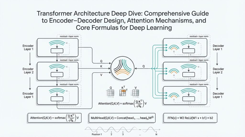
Think of the model as a two-part workshop: an encoder that reads and compresses information, and a decoder that generates or expands on that compressed understanding. The encoder (the reader) ingests the input and produces a set of internal representations; the decoder (the writer) takes those representations and produces the output step by step. Treating them as separate but cooperating teams gives us the encoder–decoder structure, which is ideal when you need to convert one sequence into another — for example, translating English to Spanish. Building on that cooperative idea helps us design systems that are modular and easier to scale.
To make the cooperation work, we rely on self-attention, which is the mechanism that lets every token (a word or piece of a word) look at every other token and decide what’s important. Self-attention means each element creates three vectors called a query (what it’s looking for), a key (what other elements offer), and a value (the content to be passed along). The model compares queries to keys to compute weights, then uses those weights to mix the values into a context-aware representation. You can think of it like shopping: your query is a grocery list, keys are product labels, and values are what you actually buy — the matching process determines what ends up in your cart.
We make this process richer with multi-head attention and positional encoding. Multi-head attention runs several attention “detectors” in parallel so the model can examine relationships from multiple perspectives (like having several people each notice different patterns in the same paragraph). Positional encoding is how we tell the model where tokens sit in a sequence — because attention by itself is order-agnostic. Positional encodings add a sense of sequence — like timestamps on photos — so the model knows whether a word comes before or after another, which is crucial for meaning in language.
Architectural principles guide the Transformer’s design: keep modules modular, enable parallel computation, stabilize training, and allow depth to grow. Modularity means attention, feed-forward layers, normalization, and residual connections are cleanly separated so we can tweak or scale parts individually. Parallelism comes from processing tokens simultaneously instead of step-by-step, which accelerates training on modern hardware. Stability tricks such as layer normalization and residual connections help gradients flow through deep stacks so we can train very large models without losing signal.
So what does this mean in practice as we move deeper into formulas and implementation? It means we can focus on a few core building blocks — queries/keys/values, scaled dot-product weighting, softmax normalization, and stacking attention with feed-forward layers — and reason about how changing dimensions, heads, or depth affects capacity and speed. As we proceed, we’ll unpack the precise computations and trade-offs that let a Transformer scale from a tiny proof-of-concept to a production-sized model, and we’ll show how those choices shape real-world performance.
Encoder-Decoder Stack Architecture Layer Roles
Imagine you’ve built the first blocks of a Transformer and now you’re peering into the stack asking: who does what? Right up front, the encoder-decoder partnership drives everything — the encoder compresses the input into rich signals and the decoder expands those signals into an output sequence. We’ll use the terms encoder-decoder, Transformer, and attention mechanisms often, because they map directly to the roles each layer plays. Think of layers as team members in a relay race: each takes the baton, adds something, and hands it on with a clearer signal.
Let’s meet the cast of layer types you’ll see in each stack position. Embeddings turn tokens into vectors (numbers that capture meaning), and positional encodings add sequence order so the model knows who came first. Self-attention (where tokens compare queries, keys, and values) is the scout that finds relationships across the whole input, while feed-forward layers — simple neural nets applied to each position — are the local craftsmen that refine features. Residual connections and layer normalization are the support crew that keep training stable and let deeper stacks learn without losing information.
In the encoder, each layer’s job is to enrich and compress the input into context-rich representations. The topic sentence is simple: encoder layers read broadly and summarize repeatedly. Self-attention here (self-attention = tokens looking at every other token) lets each token gather context from the whole sequence, so a word’s representation becomes informed by long-range dependencies. The feed-forward sublayer then transforms those contextual signals into more expressive features, while residuals and normalization protect and regularize the signal so depth actually helps instead of harms.
On the decoder side, layer roles shift toward selective generation and controlled reading of encoder outputs. The decoder’s masked self-attention enforces causality (masked self-attention means each position can only see earlier positions), which keeps generation step-by-step during inference. Then cross-attention allows the decoder to query the encoder’s representations — in other words, the decoder asks the encoder “what do you know about this part?” and selectively pulls that information in. Finally, a feed-forward stage sharpens the combined signal into the token prediction space, turning raw context into a candidate word distribution.
Stacking these layers is where representation refinement becomes a story arc: earlier layers capture surface patterns and syntactic links, middle layers form compositional features, and deeper layers tend to carry higher-level, task-specific semantics. Multi-head attention (multiple parallel attention detectors) spreads attention mechanisms across different perspectives so one head might track subject-verb agreement while another follows coreference. Residual paths make sure lower-level detail remains available higher up, allowing the decoder to mix raw and abstract signals when producing outputs. This layered refinement is why depth often improves performance: each layer adds a pass of “reasoning” over the sequence.
So what does this mean when you design or debug a model? Start by asking which layer needs more capacity: do you need wider feed-forward layers for richer per-token processing, or more attention heads so the model can examine relationships from more viewpoints? Increasing encoder depth helps when input complexity is high; strengthening decoder cross-attention helps when alignment between input and output is crucial. Keep these roles in mind as you tune: the encoder reads and compresses, attention mechanisms connect ideas, and the decoder reads selectively to generate — and that mental map will guide sensible architectural changes as you iterate.
Scaled Dot-Product Attention Mechanics and Intuition
Imagine you’ve got a question about a sentence and want the model to look through every word to find the ones that matter — that’s where the scaled dot-product attention and the broader attention mechanism step in. Picture each token producing three helpers called queries, keys, and values: the query asks a question, the key describes what each token offers, and the value is the content we might borrow. Building on what we already learned about encoder–decoder roles, this operation is the lightweight, highly parallel way the model decides how much of each value to mix into a token’s new representation.
First, think of the dot product as a measure of agreement: when a query and a key point in similar directions, their dot product is large and the token should be listened to more closely. This geometric idea is intuitive — dot product equals how well two vectors align — but when dimensions grow, those raw numbers can balloon. To keep things stable we divide by the square root of the key dimensionality (d_k); that scaling shrinks the numbers so the next step behaves well. How do you choose that scale? In practice we use sqrt(d_k) because it counteracts the expected growth of dot products as vector length increases, preserving meaningful gradients during training.
Now let us walk through the computation as a short recipe so you can picture it step by step. First we multiply the matrix of queries by the transpose of the keys to get a matrix of pairwise scores (this is the fast, parallel part). Then we divide each score by sqrt(d_k) to normalize magnitudes. Next we apply softmax — a function that turns scores into positive weights that sum to one, like a probability distribution — so stronger matches get larger weights. Finally we multiply those weights by the matrix of values to produce the context-aware outputs you feed forward in the network.
To make the intuition concrete, imagine you’re at a potluck and each guest (a token) holds up a small sign listing what they can contribute (the key) and a box of food (the value). Your query is your craving: you compare your craving to everyone’s sign (dot product), scale your enthusiasm so you don’t overcommit, then turn those comparisons into a set of probabilities (softmax) that say how much of each box you sample. If you had very long signs with many details, the raw matches might overwhelm you — scaling is the calm, sensible friend who keeps decisions from becoming extreme.
This computational pattern matters because it shows up everywhere: self-attention (tokens attending to tokens within the same sequence) and cross-attention (decoder queries attending to encoder outputs) both use the same scaled dot-product core. The scale stabilizes training, softmax gives interpretable weights, and the whole pattern is cheap to compute with matrix multiplication libraries on GPUs. A practical takeaway: the key dimension d_k is usually set to the model dimension divided by the number of attention heads, so when you split attention into multiple heads you preserve per-head scale while letting each head focus on different relationships.
With that understanding in hand, we’re ready to see why multiple heads add power: they run several scaled dot-product attention detectors in parallel, each with its own view of queries, keys, and values, and then recombine their outputs. This is where the single-head intuition we just built becomes a small toolkit you can duplicate and mix — and it’s the natural next step when you want the model to notice several patterns at once.
Multi-Head Attention Implementation Details and Benefits
Imagine you’re trying to teach a model to notice several different patterns in the same sentence — subject–verb agreement, which nouns refer to the same entity, and which words signal sentiment — all at once. In practice we give the model a little committee to solve that problem: multi-head attention, a mechanism that runs several separate attention “detectors” (attention heads) in parallel so each can focus on a different relationship. Think of each head as a specialist at a dinner table: one tastes for spice, another for texture, and together they create a fuller review than any single palate could.
Building on the scaled dot-product attention recipe we already discussed, the implementation detail that makes multi-head attention efficient is projection and parallelism. First we apply learned linear projections to the input to produce H sets of queries, keys, and values (H is the number of attention heads). Each set has reduced dimensionality — typically d_k = d_model / H — so each head runs scaled dot-product attention in a lower-dimensional subspace. After computing attention outputs for each head in parallel, we concatenate those outputs and pass them through one final linear projection to mix the head-specific signals back into the model dimension.
A key implementation point is how these operations map to matrix math and hardware. Instead of looping over heads, you implement the projections as big linear layers that produce a single tensor shaped (batch, seq_len, H, d_k), then reshape and perform a batched matrix multiplication to compute all head attention scores at once. This keeps computation friendly to GPUs and avoids costly Python-level loops. Because each head uses smaller vectors, the per-head dot products are cheaper, and the whole multi-head block remains roughly the same order of compute as a single wide attention with smarter representational capacity.
Why split into multiple attention heads instead of one wider head? How does splitting attention into multiple heads help? The short answer is that separate heads let the model examine different linear projections (subspaces) of tokens simultaneously, so one head can latch onto syntactic cues while another captures semantic roles. There’s a practical trade-off: increasing H gives more diverse perspectives but reduces d_k unless you increase d_model; too many tiny heads can become noisy, while too few heads may miss subtle patterns. Choosing H is therefore a balance between diversity and per-head representational power.
To make this concrete, imagine reading a paragraph with several colored highlighters. Each highlighter (attention head) follows a different rule: yellow marks names, blue marks actions, green marks sentiment words. When you stack those highlighted views, you see the text’s structure more clearly than with one color alone. That’s exactly what concatenation and the final linear projection do: they recombine the specialized views into a richer token representation that subsequent layers can use.
When you implement multi-head attention in code, a few practical tips make a big difference. Always scale queries by sqrt(d_k) inside each head to stabilize gradients; use efficient fused kernels or batched GEMM to avoid memory-bound loops; and for autoregressive decoding cache past keys and values per head so you don’t recompute them at every step. Also be mindful of masking: causal (autoregressive) masks apply per head when decoding, and attention masks for padding should be broadcast across heads so each detector ignores padded positions consistently.
Taken together, multi-head attention gives you parallel, diverse, and hardware-friendly attention computation that boosts expressiveness without an exponential cost in compute. As we move forward, we’ll use this modular intuition to inspect how attention heads specialize across layers and how cross-attention mixes encoder signals into decoder generation, so we can tune head counts and dimensions with purpose rather than guesswork.
Positional Encoding Techniques and Variants
Imagine you’re teaching a model to read a sentence but the model can’t tell which word came first — that’s exactly the problem positional encoding solves. Positional encoding is a way to add order information to token vectors (a token is a unit of text like a word or subword), so the attention mechanism — which by itself treats tokens as an unordered set — can understand sequence. Early options split into two broad camps: fixed, hand-crafted signals like sinusoidal encodings, and learned embeddings where the model picks a position vector during training. How do you choose between these approaches when building an encoder–decoder system or a generator model?
First, let’s meet the sinusoidal family. Sinusoidal positional encodings use sine and cosine waves at different frequencies to produce a unique pattern for each position; think of them like a set of overlapping clocks that, together, indicate a timestamp. This fixed scheme gives the model a smooth sense of distance and often helps with extrapolation beyond training lengths because the functions extend naturally. The intuition is geometric: nearby positions produce similar wave patterns, and linear shifts in position correspond to predictable phase changes — useful when you want models that generalize to longer sequences than seen at training time.
In contrast, learned positional embeddings let the model discover a vector for each absolute position during training, much like learning a word embedding. Learned embeddings can be more flexible and often improve performance on tasks where contexts are bounded and sequence lengths are consistent, because the model tailors the positional signals to the dataset. The trade-off is that learned absolute positions do not naturally extrapolate: if you suddenly ask the model to handle longer inputs than during training, those new positions have no learned vectors and the model can struggle.
Taking this idea further, relative positional encoding focuses on the distance between tokens rather than their absolute indices. Relative positional encoding (where the model learns to represent relative offsets) helps in tasks where relationships — how far apart two words are — matter more than absolute position, such as coreference or alignment-heavy translation. Practically, relative schemes add learned biases or modify attention scores based on token distances, which often improves handling of variable-length inputs and reduces sensitivity to sequence truncation.
More recent variants mix creativity with mathematical tricks. Rotary positional embeddings (RoPE) encode position by rotating query and key vectors in a way that injects relative phase differences; you can think of RoPE as applying a tiny rotation to each vector so that dot-product similarity implicitly encodes distance. Another lightweight idea is ALiBi (Attention with Linear Biases), which adds a simple linear bias to attention scores to prefer nearer tokens; ALiBi is appealing for its simplicity and strong empirical ability to extend to longer contexts without retraining. These options often excel in autoregressive generation or long-context tasks because they impose a distance-aware inductive bias directly inside attention computations.
So what should you pick in practice? If you expect fixed-length inputs and want the highest task-specific accuracy, learned positional embeddings are a solid choice. If you need generalization to longer contexts or you’re building an autoregressive decoder where caching past keys/values matters, relative encodings, RoPE, or ALiBi are typically better. Consider compute and implementation constraints too: some relative schemes change attention’s shape and require careful batching, while RoPE and ALiBi integrate cleanly with cached decoding and are memory-friendly.
Imagine we’re building a document summarizer: if our documents vary widely in length and we want the model to generalize to longer pieces, we’d likely pick RoPE or ALiBi and validate by testing on longer held-out documents. If we’re training on many short, uniformly-sized examples, learned positional embeddings could give a small performance edge. Either way, check masking compatibility (causal masks for decoders, padding masks for encoders) and measure whether your chosen encoding plays nicely with multi-head attention and caching.
Building on the attention mechanics we already discussed, positional choices are a subtle but powerful lever: they change what patterns attention finds easiest to express and how a model generalizes across sequence length. With an encoding strategy chosen, we can next examine how heads and layers specialize around those positional signals and how cross-attention uses positional cues to align input and output sequences.
Core Formulas, Derivations, and Code
Imagine you’re at the whiteboard with a Transformer and you want to see exactly what its brain is doing — not high-level metaphors, but the algebra and runnable code that brings those ideas to life. Building on our earlier intuition, the single most important formula you’ll meet is the scaled dot-product attention, which takes matrices of queries (Q — what each token is asking for), keys (K — what each token offers), and values (V — the content to be mixed). The core computation is compact and powerful:
Attention(Q, K, V) = softmax( (Q K^T) / sqrt(d_k) ) V
Here the dot product Q K^T gives pairwise similarity scores; sqrt(d_k) (where d_k is the key dimensionality) scales those scores to keep gradients well-behaved; softmax turns scores into positive weights that sum to one; and multiplying by V mixes content according to those weights. Softmax is the function that exponentiates and normalizes a vector so larger scores produce proportionally larger weights; the division by sqrt(d_k) prevents very large dot products when vectors are high-dimensional, which would otherwise push the softmax into near-one-hot extremes and harm learning.
Let’s step through the shapes so you can reason about implementation. If Q has shape (batch, seq_q, d_k), K and V have shapes (batch, seq_k, d_k) and (batch, seq_k, d_v) respectively, then Q K^T yields (batch, seq_q, seq_k) — a matrix of scores for every query against every key. After softmax you still have (batch, seq_q, seq_k); multiplying by V produces (batch, seq_q, d_v), a context-aware representation for each query position. Keeping track of these shapes is how you debug attention when it doesn’t behave the way you expect.
Now let us take that core and expand it into the multi-head pattern. Multi-head attention (several attention “detectors” running in parallel) projects inputs into H heads so each head works in a d_k = d_model / H subspace, computes attention, and the heads’ outputs are concatenated and recombined. In code-like pseudocode:
# shapes: x (batch, seq, d_model)
Q = Wq(x)  # (batch, seq, H * d_k)
K = Wk(x)
V = Wv(x)
Q = Q.view(batch, seq, H, d_k).transpose(1,2)  # (batch, H, seq, d_k)
# compute attention per head in batched form
scores = Q @ K.transpose(-2,-1) / math.sqrt(d_k)
weights = softmax(scores)
out = weights @ V  # (batch, H, seq, d_k)
out = out.transpose(1,2).contiguous().view(batch, seq, H*d_k)
out = Wo(out)
This implementation note matters: instead of looping over heads in Python (slow), you reshape and use batched matrix multiplications so GPUs run everything in parallel. For autoregressive decoding (where you generate tokens one at a time), cache K and V per head to avoid recomputing them at each step — store them in shape (batch, H, cached_seq, d_k) and append new keys/values as tokens are produced.
A short derivation clarifies why scaling by sqrt(d_k) emerges naturally. If elements of Q and K are zero-mean with variance 1, their dot product has variance proportional to d_k; dividing by sqrt(d_k) normalizes the variance to a constant scale, keeping the softmax input distribution stable as we change model width. That small normalization step is what makes deep stacks of attention layers train reliably.
How do cross-attention and self-attention differ algebraically? Self-attention is the same formula with Q, K, V all derived from the same source (the same sequence); cross-attention uses Q from the decoder and K, V from the encoder, so the attention matrix aligns decoder queries to encoder keys and pulls encoder values into the decoder’s representations. This algebraic symmetry is why Transformers are modular: the same attention primitive composes both reading (encoder) and targeted querying (decoder).
Before we move on, try this quick experiment in your environment: implement the two-line attention kernel above with small random tensors, print shapes, and verify that increasing d_k without scaling makes softmax weights saturate. That hands-on check is the fastest way to internalize why the formulas are written the way they are, and it sets you up to tune head counts, d_model, and positional encoding choices with confidence.