When to Use Adam
Building on the intuition behind adaptive optimization, the Adam optimizer is your go-to when you need fast, robust convergence across heterogeneous parameter groups. Why does this matter? When your model has parameters that learn at very different scales—sparse embeddings, attention heads, or deep recurrent weights—Adam’s adaptive learning rates and moment estimates reduce manual per-parameter tuning and stabilize early training. When should you pick Adam over SGD? If you want reliable progress from noisy gradients, a small batch regime, or rapid prototyping where wall-clock time matters, Adam often wins out.
Adam combines first-moment (mean) and second-moment (uncentered variance) estimates to scale updates per parameter, which effectively implements an adaptive learning rate for each weight. This per-parameter scaling accelerates convergence on ill-conditioned objectives where curvature differs across directions, and bias-correction helps early steps behave sensibly. Because of these properties, Adam tolerates higher base learning rates and reduces sensitivity to initial hyperparameter guesses—important when you can’t run dozens of long experiments. In practice, that means fewer wasted GPU hours getting a model to reasonable loss.
You’ll see Adam pay off in concrete scenarios we encounter frequently. Fine-tuning pretrained transformers or BERT-like models with limited labeled data benefits from Adam’s stability and default lr scale (e.g., lr ~1e-5–1e-4 for fine-tuning and lr ~1e-3 when training from scratch). Training models with sparse gradients—recommendation systems with large embedding tables—or reinforcement learning agents with high reward variance also improves with Adam. In PyTorch, a common starting pattern is optimizer = Adam(model.parameters(), lr=1e-3) for prototypes, then switch to a tuned schedule for production runs.
That said, Adam is not universally optimal. For large-scale supervised tasks where final generalization is the priority—ImageNet-scale image classification being the canonical example—SGD with momentum and a carefully tuned learning-rate schedule often yields better test accuracy. Adam’s adaptive steps can implicitly regularize differently, sometimes producing worse minima for generalization. Additionally, Adam uses more memory (tracking two moments per parameter) and can complicate distributed synchronous training at extreme scale, so resource constraints or strict generalization requirements may push you toward SGD.
So how do you decide in practice? Start with Adam when you need fast iteration, your batch size is small, gradients are noisy or sparse, or you’re fine-tuning large pretrained models. Monitor the training/validation gap and stability: if validation accuracy plateaus or generalizes poorly relative to baseline expectations, try a staged strategy—train quickly with Adam, then switch to SGD with momentum for the last 10–30% of epochs while reducing the learning rate. Also prefer AdamW (decoupled weight decay) rather than the original Adam when you need proper L2 regularization. Use warmup schedules and examine learning-rate sensitivity before over-tuning other knobs.
In short, pick Adam when training stability, speed, and per-parameter adaptivity are higher priorities than squeezing out the last drop of generalization on massive, well-behaved datasets. We’ll next turn to practical hyperparameter recipes and diagnostics that make Adam behave well in production, including sensible defaults, when to adjust betas, and how to detect when an optimizer switch will help.
Intuition Behind Adam
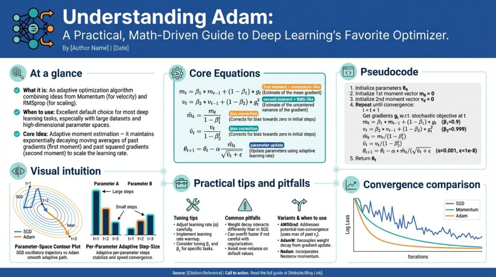
Building on this foundation, think of the Adam optimizer as two complementary instincts working together: one that remembers direction and one that measures how noisy that direction is. Right away you should front-load the idea that Adam combines momentum-like tracking (first-moment estimates) with per-parameter scale control (second-moment estimates) to produce adaptive learning rates that change for each weight. This pairing is why Adam optimizer often converges quickly on noisy or heterogeneous problems: the update direction is smoothed while the step size is scaled to local gradient variability, so you make consistent progress without large, erratic jumps.
Start with the first-moment intuition: we treat recent gradients as an exponentially weighted average, so we follow consistent directions instead of reacting to every minibatch spike. That moving average (the “m” term) is essentially momentum: it biases updates toward recent trends and reduces high-frequency noise. In contrast, the second-moment estimate (the “v” term) tracks the average squared gradient and tells us which parameters consistently see large gradients versus those that see tiny ones. Together, these moment estimates let you separate “which way to move” from “how far to move”, which is the core of per-parameter adaptivity and why adaptive learning rates feel natural in Adam.
How does bias correction fit into this picture and why is it necessary? Because we initialize both moment estimates at zero, their early values underestimate the true moments—especially with common beta values like 0.9 and 0.999—so raw m and v are biased toward zero in the first few steps. Bias-correction rescales m and v to approximate their unbiased expectations, producing sensible early updates instead of tiny, ineffective steps. Practically, that means Adam behaves robustly from step one: you can use a larger base learning rate during warmup and expect meaningful parameter movement rather than waiting for the averages to “warm up.”
If you like concise formulas to anchor intuition, the update loop shows the separation clearly: m <- beta1m + (1-beta1)g; v <- beta2v + (1-beta2)(g*g); m_hat <- m/(1-beta1^t); v_hat <- v/(1-beta2^t); theta <- theta – lr * m_hat / (sqrt(v_hat) + eps). Reading it this way, you can see m_hat supplies the signed direction and v_hat normalizes magnitude. That normalization is what gives Adam adaptive learning rates: parameters with large v_hat get smaller effective steps, and parameters with small v_hat get larger steps, automatically compensating for scale and sparsity differences across parameter groups.
For a geometric perspective, imagine an objective whose curvature varies dramatically across axes: steep along one direction, flat along another. Standard gradient descent takes the same step length in both directions, which causes zig-zagging and slow progress. Adam’s diagonal preconditioner (1/sqrt(v_hat)) approximates curvature per coordinate, shrinking steps where gradients are consistently large and stretching steps where gradients are small. This is not a full Hessian-based natural gradient, but it’s a cheap, per-parameter approximation that dramatically improves convergence on ill-conditioned problems and sparse embeddings.
Finally, use this intuition to guide hyperparameter and debugging choices. If updates oscillate, increase beta1 to smooth the direction; if learning stalls because steps are vanishingly small, check v_hat magnitudes and consider lowering beta2 or raising lr temporarily. Monitor the ratio |m_hat| / (sqrt(v_hat)+eps) across layers to see which parts of the model are effectively learning. Taking these diagnostics into account, we can pick sensible defaults and know when to adjust them; next we’ll translate this intuition into concrete hyperparameter recipes and practical diagnostics that make Adam optimizer behave well in production.
Moments and Bias Correction
Early in training the Adam optimizer often takes surprisingly small steps, and that behavior ties directly to how we initialize and use moment estimates and bias correction. When m and v start at zero they systematically underestimate the true first and second moments, which makes raw updates tiny for the first few iterations. How does bias correction change early updates? Bias correction rescales those moving averages by factors (1 – beta1^t) and (1 – beta2^t), producing m_hat and v_hat that approximate the unbiased expectations and therefore restore sensible effective learning rates right away. Front-loading this intuition helps you reason about warmup, learning-rate choices, and why Adam behaves robustly from step one.
The first moment (m) acts like momentum: it accumulates gradient direction, while the second moment (v) measures gradient magnitude. Because m_t = beta1 * m_{t-1} + (1 – beta1) * g_t and v_t = beta2 * v_{t-1} + (1 – beta2) * g_t^2 start at zero, their expectations include multiplicative factors (1 – beta1^t) and (1 – beta2^t). Dividing m and v by those factors—m_hat = m / (1 – beta1^t), v_hat = v / (1 – beta2^t)—removes the startup bias so that the numerator supplies an unbiased direction and the denominator supplies an unbiased scale estimate. That unbiased pairing is what enables Adam to implement per-parameter adaptive learning rates reliably from iteration one.
To see the quantitative impact, consider common defaults beta1=0.9 and beta2=0.999. After the first step 1 – beta1^1 = 0.1, so m is scaled up by 10x; for v, 1 – beta2^1 = 0.001, so the uncorrected v is vanishingly small and would otherwise make the denominator artificially large after sqrt, producing tiny steps. Bias correction reverses this and prevents Adam from effectively “stalling.” In practice you’ll notice that disabling bias correction or using poor beta choices produces either excessive early oscillation or grindingly slow warmup—exactly the pathologies we want to avoid when tuning adaptive learning rates.
What does this mean for hyperparameter decisions and diagnostics? First, keep bias correction enabled unless you have a deliberate experimental reason to disable it. If training appears stuck in the first few epochs, log layer-wise statistics like m_hat, sqrt(v_hat), and the step magnitude ratio r = |m_hat| / (sqrt(v_hat) + eps); consistently near-zero r indicates startup bias or overly large beta2. Second, if v_hat grows too quickly and suppresses updates, consider lowering beta2 (e.g., 0.99) to make the variance estimate more responsive, but be aware this increases noise sensitivity. These checks translate directly into actionable adjustments rather than blind hyperparameter sweeps.
We can also use small code patterns to inspect and validate moment behavior during a run. For example, compute m_hat = m / (1 – beta1t) and v_hat = v / (1 – beta2t) inside your training loop and emit percentiles for each parameter group every N steps; watching the 50th and 90th percentiles of r = |m_hat|/(sqrt(v_hat)+eps) reveals which layers are effectively learning. For sparse embeddings you’ll often see high variance in v_hat and correspondingly larger adaptive learning rates for rare tokens, which is the intended adaptive behavior. Instrumentation like this turns abstract math into concrete signals you can act on.
Taking this concept further, bias correction connects to practical strategies like learning-rate warmup and optimizer switching. Because bias correction fixes the initial underestimation but not the noise characteristics of gradients, you may still prefer a short warmup to avoid large initial updates when using high base lrs. Conversely, if you plan to switch from Adam to SGD late in training, validate that m_hat magnitudes have decayed and that v_hat has stabilized so the transfer of momentum and scale properties is predictable. By treating moment estimates and bias correction as measurable first-class diagnostics, we can make optimizer choices that are explainable, reproducible, and tuned to the real behavior of our models.
Update Rule Derivation
We start from a practical question: how does the Adam optimizer transform raw stochastic gradients into the per-parameter steps you actually apply? Building on the intuition about moments and bias correction we already discussed, the derivation shows exactly why Adam uses exponential moving averages, why we correct their startup bias, and why the denominator uses a square root plus epsilon. This gives you a concrete algebraic bridge from g_t (the minibatch gradient) to the adaptive update used in frameworks.
Begin with plain stochastic gradient descent: a parameter update is theta_{t+1} = theta_t – alpha * g_t, where g_t = \nabla_theta L(\theta_t) and alpha is the global learning rate. To get adaptive learning rates we introduce a diagonal preconditioner D_t so the step becomes -alpha * D_t * g_t; the derivation of Adam picks D_t from running statistics of gradients so each coordinate rescales independently. This framing—gradient times a diagonal preconditioner—lets us interpret Adam as a cheap, per-parameter curvature approximation that yields adaptive learning rates.
Next, define the two exponential moving averages that capture direction and scale: m_t = beta1 * m_{t-1} + (1 – beta1) * g_t and v_t = beta2 * v_{t-1} + (1 – beta2) * (g_t * g_t). These recurrences implement exponentially weighted estimates of the first and second (uncentered) moments of the gradient. Because both m and v initialize at zero they are biased toward zero for small t; we therefore compute bias-corrected forms m_hat_t = m_t / (1 – beta1^t) and v_hat_t = v_t / (1 – beta2^t) so the expectations match the true moments early in training. That bias correction is essential to make early updates meaningful rather than vanishingly small.
Now form the update rule from those corrected moments. We want a signed direction from the first moment and a scale from the second, so Adam uses the rule theta_{t+1} = theta_t – alpha * m_hat_t / (sqrt(v_hat_t) + eps). Why this specific algebraic shape? Because m_hat_t approximates E[g] (a directional signal) while sqrt(v_hat_t) approximates the RMS magnitude of g (an amplitude signal); dividing by the RMS normalizes step lengths across coordinates. The small constant eps avoids division by zero and controls sensitivity when v_hat_t is tiny. Together, that expression implements adaptive learning rates per parameter while retaining a momentum-like smoothing in the numerator.
It helps to view this as a diagonal preconditioner: D_t ≈ diag(1 / (sqrt(v_hat_t) + eps)). In second-order terms, a full Newton step would multiply by H^{-1}g, but Adam uses a cheap diagonal approximation built from gradient second moments rather than curvature—effectively trading exact curvature for computational efficiency and stability. This also clarifies relationships: RMSProp supplies the v-based normalization, classic momentum supplies the m-based direction, and Adam blends both with bias correction to produce stable adaptive learning rates. Keep in mind this is an approximation, so for ill-conditioned problems a full-matrix method or a carefully scheduled SGD may still be preferable.
What are the practical knobs that follow from the derivation? Because v_hat appears under a square root, beta2 controls how rapidly the per-parameter scale adapts—high beta2 (=0.999) produces very smooth v estimates and small initial denominators that must be bias-corrected; lowering beta2 (e.g., toward 0.99) makes v_hat respond faster but adds noise. The ratio r_t = |m_hat_t| / (sqrt(v_hat_t) + eps) is the effective step magnitude for each coordinate and is the diagnostic you should log when debugging. By deriving the update rule this way we see why bias correction, eps, and the two betas matter, and how the Adam optimizer produces the adaptive learning rates that make it robust across heterogeneous parameter groups. Building on this derivation, we’ll next translate these algebraic choices into hyperparameter recipes and practical diagnostics you can run in training.
Hyperparameters and Tuning
Tuning the Adam optimizer often determines whether a run converges cleanly or drifts into noisy plateaus; front-load your attention on the base learning rate and a couple of companion knobs and you’ll save hours of iteration. Building on the earlier intuition about first- and second-moment estimates, start by treating the global learning rate as the most sensitive hyperparameter: it multiplies the effective per-parameter step r_t = |m̂|/(sqrt(v̂)+eps). How do you pick a starting value for learning rate when your model and data differ dramatically? Use a short logarithmic sweep (e.g., 1e-6 → 1e-1) over a few hundred iterations to find the range where loss consistently decreases, then refine within that band.
Once you’ve located a viable learning rate range you’ll want concrete defaults to iterate from. For most prototypes, initialize with AdamW rather than legacy Adam so weight decay is decoupled from adaptive updates; try lr in 1e-3–1e-4 for training from scratch and 1e-5–1e-4 for fine-tuning pretrained transformers, with weight_decay ≈ 1e-2 and eps = 1e-8. Keep beta1 close to 0.9 to retain momentum smoothing and beta2 near 0.999 for a stable variance estimate; these defaults work widely, but treat them as starting points to be validated by diagnostics rather than immutable rules.
If training stalls or effective steps collapse, adjust the betas and eps strategically rather than sweeping blindly. Lowering beta2 (for example to 0.99) makes the v estimate more responsive and can rescue models where sqrt(v̂) grows too large and suppresses progress, but it increases variance in step sizes. Increasing eps (e.g., to 1e-6) can stabilize mixed-precision or very small-gradient regimes by preventing division issues. We recommend monitoring the percentile statistics of r_t across parameter groups: persistent near-zero medians signal an over-large beta2 or a learning rate that’s too small.
Warmup and learning-rate schedules are complementary tuning levers you should leverage for stability and generalization. Use a short linear warmup for the first 1–5% of total steps when your base learning rate is high or when fine-tuning large pretrained models, then switch to a decaying schedule—cosine annealing or step decay are both viable depending on epoch budget. If your goal is ultimate generalization and you’ve trained quickly with Adam, consider switching to SGD with momentum for the final 10–30% of epochs while annealing the rate; this staged approach often combines Adam’s fast convergence with SGD’s generalization during the final descent.
Instrumentation is how tuning becomes science instead of guesswork. Log layer-wise and parameter-group percentiles for |m̂|, sqrt(v̂), gradient norm, and the effective per-parameter LR = lr * |m̂|/(sqrt(v̂)+eps). A simple pattern in your training loop is to emit the 10th, 50th, and 90th percentiles of r_t every N steps and correlate those with validation loss changes; this shows which layers are learning and which are effectively frozen by the denominator. When you identify problematic layers, treat them with per-parameter-group overrides—lower lr for embeddings, increase lr for randomly initialized heads, or apply different weight_decay values—rather than global blind adjustments.
Finally, watch for common practical pitfalls and apply a short checklist during experiments: default to AdamW, run an initial learning-rate sweep, use modest warmup, log r_t percentiles, and only then tweak betas or eps. For mixed-precision training bump eps slightly and validate that moment statistics remain well-scaled; for sparse embeddings accept larger v variance and compensate with per-group learning rates. These diagnostics and tuning patterns let us translate the math of moments and bias correction into repeatable recipes so your use of the Adam optimizer yields faster convergence and more predictable behavior in production training runs.
Practical Code Example
Building on this foundation, a practical way to understand Adam’s behavior is to instrument the optimizer and inspect the effective per-parameter step magnitudes that implement the adaptive learning rates. How do you inspect whether Adam’s adaptive learning rates are actually helping a layer? We’ll show a small, repeatable pattern you can drop into a PyTorch loop to compute bias-corrected first and second moments and emit percentiles that reveal which parameters are learning and which are being suppressed by the denominator.
The code below uses PyTorch’s AdamW state internals (exp_avg and exp_avg_sq) to compute m̂ and v̂ and then the effective step r = |m̂|/(sqrt(v̂)+eps). Insert this after optimizer.step() and before zero_grad() so state[‘step’] is up to date:
# inside training loop, after optimizer.step()
import torch
def log_adam_stats(optimizer, tag="train"):
    stats = {}
    for i, group in enumerate(optimizer.param_groups):
        r_vals = []
        for p in group['params']:
            state = optimizer.state[p]
            if 'exp_avg' not in state:
                continue
            m = state['exp_avg']
            v = state['exp_avg_sq']
            t = float(state.get('step', 1))
            beta1, beta2 = group.get('betas', (0.9,0.999))
            m_hat = m / (1 - beta1**t)
            v_hat = v / (1 - beta2**t)
            r = (m_hat.abs() / (v_hat.sqrt() + group.get('eps',1e-8))).flatten()
            r_vals.append(r)
        if not r_vals:
            continue
        r_all = torch.cat(r_vals)
        stats[f'group_{i}_p50'] = r_all.quantile(0.5).item()
        stats[f'group_{i}_p90'] = r_all.quantile(0.9).item()
    print(tag, stats)
This pattern computes the same m̂ and v̂ used in the optimizer update and produces the effective per-parameter LR when multiplied by the group lr. Use the p50/p90 percentiles to quickly spot layer imbalance: a very low median indicates parameters are effectively frozen by large v̂, while a high p90 with a low median shows a few outlier parameters dominating updates. Logging these values every N steps turns opaque optimizer dynamics into actionable diagnostics and helps you decide whether to change lr, beta2, or per-group settings.
For a concrete example, when fine-tuning a transformer you’ll often see heads and classifier layers with high r percentiles while large token embedding matrices have tiny medians. In that case keep AdamW as the optimizer, but apply per-parameter-group overrides: increase the lr for newly-initialized heads, reduce the lr for embeddings, and keep weight_decay off for bias and LayerNorm. If you observe tiny r across the board early in training despite bias correction, check step counts and consider a short linear warmup (500–2000 steps) or temporarily lower beta2 (e.g., 0.99) so v̂ adapts faster.
Mixed-precision and distributed setups change the practical knobs slightly. In AMP runs increase eps from 1e-8 to 1e-6 to avoid catastrophic scaling when v̂ is tiny; ensure gradient scaling is disabled during the instrumentation step or unscale gradients before reading state. When switching optimizers mid-training (for example, to SGD with momentum for final fine-tuning), transfer any learning-rate schedule state and reset momentum buffers explicitly so the new optimizer starts from a predictable state rather than inheriting incompatible momentum statistics.
Instrumenting Adam like this turns heuristic tuning into measurement-driven decisions. Rather than guessing whether adaptive learning rates or bias correction are helping, you’ll have concrete percentiles and trends to guide changes to lr, betas, eps, and per-group configurations. Next, we’ll translate these diagnostics into repeatable hyperparameter recipes and experiment patterns you can run to automate sensible defaults and optimizer switches.
