What Bias and Variance Mean
Building on this foundation, think of a machine learning model as a map trying to represent a real landscape. Bias and variance are the two main ways that map can miss the terrain. Bias is the model’s built-in tendency to lean in the wrong direction because its assumptions are too simple, while variance is the model’s tendency to wobble when the training data changes. If you have ever wondered, “Why does one model look brilliant on the data I trained it on but struggle on fresh examples?”, bias and variance are the answer we need.
Bias is the more predictable kind of mistake, which makes it feel a little like a shortcut that went too far. When a model has high bias, it is so constrained that it cannot capture the real pattern in the data, so its average prediction stays far from the true relationship. MIT’s explanation frames bias as the gap between the true function and the average prediction the model would make across many training sets. A straight line trying to describe a curving road is a good everyday picture: the line is stable, but it is too simple to follow the actual shape.
Variance is the opposite problem. A high-variance model changes too much when you give it a different sample of training data, as if it is listening to every tiny whisper in the room instead of the main conversation. That makes it sensitive to noise, which is just random variation in the data that does not reflect the real pattern we want to learn. MIT notes that variance measures how much predictions spread around their average, and that more complex models often have higher variance because they can fit noise more closely. In practice, this is why a model can look impressive on one dataset and then behave differently on the next.
Now the bias-variance tradeoff starts to make sense. When we make a model more flexible, it usually becomes better at fitting the training data, so bias goes down, but variance often goes up because the model becomes more sensitive to the exact sample it saw. When we make a model simpler, the pattern flips: variance tends to fall, but bias tends to rise. Stanford’s machine learning materials describe this as a balance between methods that are more stable across training sets and methods that can capture more complicated decision boundaries, which is why there is no single universally best model for every problem.
This is where regularization enters the story. Regularization is a way of adding a penalty or constraint during training so the model does not become too wild, much like putting guardrails on a winding road. MIT explains that you can tune a regularization strength parameter to change the balance between bias and variance, and that there is often an optimal middle point where total test error is lowest. In plain language, regularization may raise bias a little, but it can reduce variance enough to improve how well the model performs on new data.
So if your model scores well on training data but disappoints on new data, you are often looking at high variance. If it misses the pattern almost everywhere, it is usually carrying too much bias. The goal is not to erase one side completely, because that usually makes the other side worse; the goal is to find the balance where the model learns enough of the real pattern without becoming overly sensitive to noise. That balance is the heart of the bias-variance tradeoff, and once that clicks, the next step is learning how to spot it in practice.
Underfitting vs Overfitting
Building on this foundation, imagine the next scene in your model-building story: one version seems to miss the obvious pattern no matter how long you train it, while another looks brilliant on the examples it has already seen but starts to stumble the moment fresh data arrives. Those are the two classic failure modes we are trying to avoid. An underfit model is too weak to learn the structure in the data, while an overfit model learns too much of the training set, including the random noise that should have been ignored. In practice, both problems hurt generalization, which is the model’s ability to perform well on new data.
Underfitting usually shows up when the model is too simple for the task, or when its built-in assumptions are too restrictive. Think of it like trying to explain a detailed map with a single straight road: the shape is there, but the important turns and curves are missing. In machine learning terms, the model has too much bias, meaning it leans in a fixed direction and cannot bend enough to capture the real relationship between features and labels. That is why an underfit model can perform poorly even on the training data, not just on new examples.
Overfitting feels almost like the opposite story. Here, the model has enough flexibility to memorize the training set, but that flexibility becomes a trap because it also starts treating noise as if it were signal. A useful way to picture this is a student who copies every mark on a page instead of learning the lesson underneath it. The training score looks impressive, but the test score drops because the model has learned details that do not repeat outside that one dataset. This is why complex models, especially when they fit noise very closely, can look strong during training and then fail to generalize.
How do you tell which one you are seeing? The training and validation curves give away the answer. If both training performance and validation performance are low, the model is probably underfitting, because it is not learning enough from the data in the first place. If training performance keeps improving while validation performance stalls or gets worse, that gap is a strong sign of overfitting. Google’s guidance on loss curves makes this pattern very clear: the curves start together, then split when the model begins to memorize instead of generalize.
This is where the bias-variance tradeoff becomes more than a theory. When you increase model complexity, you usually lower bias but raise variance; when you simplify the model, you usually lower variance but raise bias. That is why there is no magical model that wins every time. The real goal is to find the point where the model is expressive enough to learn the pattern, but not so flexible that it chases every fluctuation in the data. Regularization and early stopping are two common ways to nudge the model back from overfitting, often with help from a validation set.
Once you can recognize these two behaviors, your next decisions become much clearer. If the model is underfitting, you may need more expressive features, a richer model, or less restrictive assumptions. If it is overfitting, you may need to simplify, add regularization, or stop training sooner. That shift from guessing to diagnosis is a big milestone, because now you are not just training a model — you are learning how to steer it toward the balance where it can actually generalize.
Model Complexity and Error
Building on this foundation, model complexity and error start to feel less like abstract classroom terms and more like a practical steering wheel. When you increase model complexity, you give the model more freedom to fit patterns in the data, but you also invite it to chase noise if you push too far. That is why the bias-variance tradeoff matters so much in machine learning: the same knob that helps a model learn can also make it fragile. If you have ever wondered, “Why does a more powerful model not always perform better?”, this is the question we are really answering.
Think of complexity like the number of moves a dancer is allowed to make. A simple model has a small set of steps, so it may miss the rhythm of a complicated song. A more complex model can move with far more detail, but if the music is messy, it may start matching every random beat instead of the real melody. In machine learning, that extra freedom can lower training error, which is the amount of mistake the model makes on the data it saw during learning. The catch is that lower training error does not guarantee lower error on new data, and that is where the story becomes interesting.
So how do you know when a model has crossed from helpful flexibility into harmful complexity? We usually look at error on both the training set and the validation set, where the validation set is a separate slice of data used to check how well the model generalizes. As the model becomes more complex, training error often keeps dropping because the model can fit the training examples more closely. Validation error, however, may fall at first and then begin to rise once the model starts fitting noise instead of signal. That turning point is the clearest sign that complexity has gone from an advantage to a liability.
This is where the familiar shape of the tradeoff appears. Very simple models tend to have high error because they cannot capture the structure in the data, which is another way of saying they are underfitting. Very flexible models can drive training error very low, but they may create a wider gap between training and validation performance, which is a classic overfitting pattern. The best model complexity is often not the one that looks most impressive on training data; it is the one that keeps validation error low enough to suggest the model has learned the real pattern rather than memorizing examples.
A useful way to picture this is a map drawer choosing how much detail to include. If the map is too plain, you miss important roads and landmarks. If it is too detailed, you may clutter the page with every tiny path, puddle, and crack in the pavement until the map becomes harder to trust. Machine learning works the same way. The right level of model complexity gives you enough detail to represent the world faithfully, while keeping the error low on data the model has never seen before.
This is also why the bias-variance tradeoff is so central in practice. As complexity rises, bias usually falls because the model can fit the data more closely, but variance usually rises because the model becomes more sensitive to the exact training sample. As complexity falls, the opposite happens: variance drops, but bias rises. Understanding that pattern helps you read error curves with more confidence, because you are no longer treating training error as the whole story. You are watching how error behaves as the model learns, and that tells you whether you are moving toward better generalization or toward a model that only looks good on paper.
Once you start thinking this way, model complexity stops feeling like a vague idea and starts acting like a decision you can manage. You are not asking, “Is this model large or small?” You are asking, “Is this the level of complexity that keeps error low where it matters most?” That shift in perspective is one of the biggest steps in learning how to build models that work in the real world.
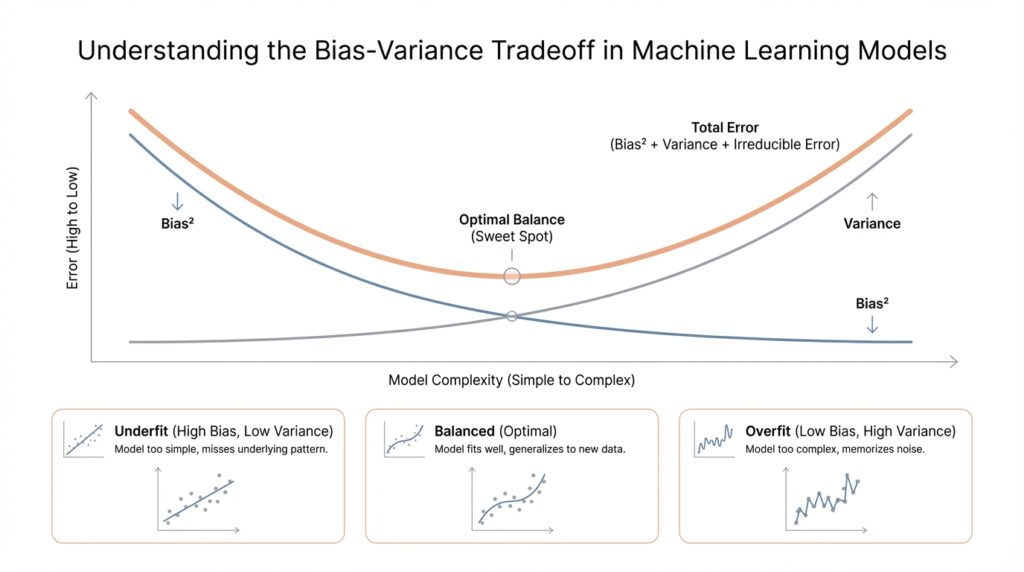
The Bias-Variance Curve
Building on this foundation, the bias-variance curve gives us a picture of how a model changes as we turn the complexity knob. Imagine we start with a very simple model and then slowly give it more freedom: first it can only draw straight lines, then curves, then highly flexible shapes. At each step, we can watch how the model’s errors shift, and that story is often more useful than a single score. How do you know when a model has enough flexibility without becoming unstable? The curve helps answer that by showing the tradeoff between learning the pattern and chasing the noise.
At the beginning of the curve, simple models usually have high bias and low variance. They are predictable, but they miss important structure because they cannot bend enough to match the data. This is why their training error and validation error both tend to stay high: the model is underfitting, and more training will not fix a design that is too rigid. Think of it like trying to sketch a mountain range with a ruler. You may draw something neat and stable, but the shape will never feel like the real landscape.
As we move along the curve and increase model complexity, something encouraging happens. The model becomes more capable, so bias drops and training error usually falls. This is the middle stretch where the model starts capturing real relationships instead of forcing everything into a narrow assumption. Validation error often improves here too, because the model is learning useful structure, not memorizing examples. In practical terms, this is the sweet spot we are hoping to find when we tune a machine learning model.
But the curve does not keep improving forever. If we keep making the model more flexible, we eventually reach a point where variance begins to climb sharply. The model starts reacting to tiny quirks in the training set, and validation error can stop falling or even rise. This is the moment when the bias-variance curve turns from a helpful guide into a warning sign. The model may look brilliant on the data it has already seen, but its generalization weakens because it has started treating noise like signal.
That shape is the reason the curve matters so much in real work. We are not looking for the most complicated model or the simplest model; we are looking for the model complexity that keeps total error as low as possible on new data. In many cases, that means aiming for the bottom of the curve, where the drop in bias still outweighs the rise in variance. This is also why regularization matters so much: it nudges the model away from the far-right side of the curve, where flexibility becomes fragility.
If you are wondering what this looks like during model selection, the answer is usually in the training and validation curves. A model that is too simple will show high error on both sets, while a model that is too flexible will show a widening gap between them. The bias-variance curve gives those numbers a shape, and that shape makes the decision easier to read. Instead of asking whether a model is “good” in the abstract, you can ask where it sits on the curve and what kind of error it is likely to make next.
Taking this concept further, the bias-variance curve becomes a kind of map for your choices. It reminds you that every gain in flexibility has a cost, and every simplification has a tradeoff of its own. Once you start reading models this way, you are no longer guessing at why performance changes. You are watching the curve tell you whether the model needs more capacity, less capacity, or a gentler balance between the two.
Common Ways to Reduce Error
Building on this foundation, the common ways to reduce error all aim at the same quiet goal: help the model learn the real pattern without becoming distracted by noise. That is the heart of the bias-variance tradeoff, and it is why people ask, “How do you reduce error in machine learning without making the model too rigid or too fragile?” We usually start by looking at the data itself, because a model can only learn from what you give it. If the input is messy, incomplete, or poorly chosen, even a strong model will struggle to generalize.
One of the first places we often look is feature engineering, which means turning raw data into inputs that are easier for a model to understand. Think of it like giving a travel map clearer landmarks instead of a blur of roads. A good feature can reveal structure that was already there, while a poor feature can hide it and force the model to work too hard. This is one of the most practical ways to reduce model error, because better features often help the model capture the signal with less strain, lowering both underfitting and overfitting risk.
If the model still feels too wobbly, regularization is usually the next tool we reach for. Regularization is a training rule that adds a penalty when the model becomes too complex, which encourages it to keep its predictions smoother and less extreme. In plain language, it acts like a governor on a fast car: you still move forward, but you avoid racing into unstable territory. This is especially useful when the model is high variance, because a small amount of extra bias can be worth it if it keeps validation error lower on new data.
Another common way to reduce error is to use cross-validation, which means testing the model across several different train-validation splits instead of relying on one lucky split. That gives you a more dependable picture of how the model is behaving, especially when your dataset is small or uneven. You can think of it as checking a recipe several times instead of trusting one tasting spoon. Cross-validation helps you compare models more fairly, choose regularization strength more wisely, and spot the point where the bias-variance tradeoff starts leaning the wrong way.
Sometimes the best fix is not to make the model fancier, but to stop it from training for too long. Early stopping is a technique where you pause training once validation performance stops improving, before the model has time to memorize the noise. This works a lot like noticing when a student has learned the lesson and no longer needs extra repetition. If you are wondering what causes a model to do well on training data but poorly on fresh examples, early stopping is often part of the answer, because it interrupts overfitting before it grows into a bigger problem.
And then there is the simplest-sounding remedy, which is often the hardest to get: more data. When you give the model a broader, more representative sample of the world, it has a better chance of learning the pattern instead of memorizing quirks from a small dataset. More data can reduce variance by making the model less sensitive to any one training set, though it does not automatically fix weak features or a poor model choice. Sometimes, the real breakthrough comes when we combine several of these approaches—better inputs, regularization, cross-validation, early stopping, and more data—so the model has a fair chance to learn well.
That is the practical side of the bias-variance tradeoff: you are not searching for one magical trick, but for the smallest set of changes that lowers error where it matters most. Sometimes the model needs more structure, sometimes less, and sometimes it just needs cleaner information to work with. Once you start thinking this way, reducing error stops feeling like guesswork and starts feeling like careful tuning, one informed adjustment at a time.
Tuning With Validation Data
Building on this foundation, validation data is where model tuning starts to feel less like guesswork and more like careful listening. After you have trained a model, you need a separate set of examples to ask a simple but powerful question: how well does this model handle data it did not memorize? That separate slice is the validation set, and it acts like a rehearsal audience before the final performance. When people ask, “How do you tune a machine learning model without fooling yourself?”, this is the place we begin.
The key idea is that validation data helps you choose settings without peeking at the final answer sheet. Those settings are called hyperparameters, which are the choices you make before or during training, such as model depth, regularization strength, or learning rate. Unlike the learned weights inside the model, hyperparameters are not learned directly from the training data. Instead, we adjust them and watch how the model behaves on validation data, looking for the version that generalizes best rather than the one that merely memorizes best.
This is where the bias-variance tradeoff becomes practical. If a model performs well on training data but starts slipping on validation data, it is usually drifting toward overfitting, which means its variance is getting too high. If both training and validation results are weak, the model is probably still too simple, which points to high bias. Validation data gives us a visible boundary between those two problems, so we can tell whether a change is helping the model learn the pattern or just helping it chase noise.
Imagine tuning a guitar before a concert. You do not want to judge the sound only by how it feels in your hands; you want to hear it from the seats where the audience will sit. Validation data plays that audience role. It tells you whether the model’s performance still sounds balanced from the outside, not just whether it feels polished during training. That is why model tuning with validation data is so valuable: it keeps our decisions tied to real-world performance, not training-room success.
So what does that look like in practice? We try a setting, train the model, measure validation performance, and compare it with the previous attempt. If validation error drops, we are moving in the right direction; if it rises, the new setting may be pushing the model too far toward complexity or too far toward simplicity. This back-and-forth is how we tune a machine learning model in a disciplined way. The goal is not to chase the lowest training error, but to find the point where validation error is lowest, because that is the strongest clue that the model will generalize.
There is one important caution here: validation data must stay clean and untouched except for tuning. If we keep checking the same validation set over and over, we can slowly start fitting to it too, which makes it less trustworthy. That is why the final test set, which is held back until the end, matters so much. The validation set helps us make choices, while the test set helps us judge those choices honestly after the tuning is done.
In many projects, validation data also helps us decide when to stop training. As training continues, the model may keep improving on the training set even while validation performance begins to stall or worsen. That gap tells us we may be crossing from useful learning into overfitting, and early stopping can step in before the model goes too far. In that sense, validation data is not just a scorekeeper; it is a guide that tells us when the model has learned enough and when more training would only make it less reliable.
Once you start using validation data this way, tuning becomes more intuitive. You are no longer asking, “Which setting looks strongest in the moment?” You are asking, “Which setting gives the model the best chance of succeeding on new data?” That small shift in perspective is what turns model tuning into a steady, thoughtful process, and it is one of the clearest ways to work with the bias-variance tradeoff instead of fighting it.