Introduction to Retail Sales Analysis with Python
The digitization of data in the retail sector has transformed the way businesses operate. Analyzing retail sales data using Python enables retailers to derive actionable insights that can help in optimizing operations, improving customer experience, and increasing profitability. Python, being a versatile programming language with a rich ecosystem of libraries, offers powerful tools for conducting detailed and comprehensive analysis of retail sales data.
To start with, retailers often face a vast quantity of data generated from various sources such as point of sale systems, customer loyalty programs, inventory management systems, and online e-commerce platforms. Python comes equipped with libraries like Pandas for data manipulation, which allows analysts to clean, filter, and segment these large datasets efficiently. With Pandas, you can easily load data from standard formats like CSV or Excel, and then perform operations such as aggregating sales figures by date or product category to identify trends and patterns.
Once the data is organized, visualization becomes crucial in drawing insights. Libraries such as Matplotlib and Seaborn enable the creation of detailed and understandable graphs. For example, a retailer can visualize the seasonality of sales using time series plots or compare the sales performance of different product lines through bar charts and heatmaps. This graphical representation of data helps in making data-driven decisions easier for stakeholders who may not be as data-savvy.
A key aspect of retail sales analysis is the ability to forecast future sales, helping businesses in inventory planning and resource allocation. Python’s Scikit-learn and Statsmodels libraries offer various statistical models and machine learning algorithms for predictive analysis. Techniques like linear regression, ARIMA models, and machine learning methods provide robust frameworks for making sales predictions.
Python’s flexibility allows for integrating this predictive capability directly into existing systems. Retailers can automate the generation of sales forecasts, which can then be compared against actual sales figures over time to refine and improve forecasting models. This iterative process of analysis and recalibration ensures that the forecasts remain accurate and relevant.
Moreover, Python supports the incorporation of advanced analytics, such as clustering and market basket analysis. These techniques are pivotal in understanding customer purchasing behavior, enabling retailers to optimize product placement and develop targeted marketing campaigns. For instance, using the Apriori algorithm available in libraries like MLxtend, retailers can identify frequently bought items together, thus strategizing on cross-selling and upselling.
In conclusion, implementing Python for retail sales analysis empowers retailers to convert heaps of data into actionable insights, aligning strategies with customer needs and market dynamics to drive growth. Leveraging Python not only enhances the analytical capabilities of a retail business but also helps in fostering a data-driven culture throughout the organization. This groundwork in using Python for retail sales analysis sets the stage for more advanced techniques and enterprise-level solutions.
Setting Up the Python Environment for Data Analysis
Setting up a Python environment for data analysis is a fundamental step for anyone embarking on a journey into retail sales analysis. This process involves installing and configuring necessary tools and libraries that facilitate efficient data manipulation, visualization, and forecasting.
To begin, ensure you have Python installed on your system. The latest stable version can be downloaded from the official Python website. Python 3 is recommended due to its enhanced features and broader library support. Once downloaded, follow the installation instructions specific to your operating system (Windows, macOS, or Linux).
After installing Python, the next essential tool is a package manager to simplify the installation of additional libraries. pip, included with Python installations, is most commonly used. Verify its installation by running pip --version in your terminal or command prompt. If not installed, you can download it by following the installation guide.
Using pip, install a virtual environment tool like venv or virtualenv. Virtual environments are crucial as they allow for isolated Python environments where you can manage dependencies specific to each project, avoiding conflicts between global and project-specific versions.
Create a virtual environment in your project directory with the command:
python -m venv env
This command creates a directory named env containing a standalone Python installation. Activate this environment using:
- Windows:
.\env\Scripts\activate - macOS/Linux:
source env/bin/activate
You should see the environment name preceding your command prompt, indicating it’s active.
Now, install the libraries essential for data analysis in retail, starting with Pandas for data manipulation. Install it with:
pip install pandas
Pandas enables quick data handling tasks such as loading datasets from CSV files, cleaning disorganized data, and facilitating operations like filtering or aggregation crucial for recognizing sales trends.
Next, install NumPy, a library for numerical computing that works seamlessly with Pandas to perform complex mathematical operations efficiently. Install it with:
pip install numpy
For data visualization, Matplotlib and Seaborn are pivotal in creating insightful plots – essential for presenting sales data visually. Install these libraries using:
pip install matplotlib seaborn
To incorporate machine learning techniques for sales forecasting, Scikit-learn is indispensable, providing tools for predictive models. Install it by running:
pip install scikit-learn
Finally, if your analysis requires statistical modeling, Statsmodels offers a variety of statistical tests and data exploration features. Install it using:
pip install statsmodels
To ensure a smooth workflow, consider using an Integrated Development Environment (IDE) such as Jupyter Notebook or VSCode. Jupyter Notebook is especially favored for data analysis due to its interactive nature, allowing code cells to run incrementally while immediately visualizing outputs. Install Jupyter Notebook using:
pip install jupyter
Start Jupyter Notebook by executing:
jupyter notebook
This command opens a web-based IDE in your browser where you can write and execute Python code, document workflows, and visualize results all in one place.
Overall, setting up this environment ensures a robust foundation not only for retail sales analysis but also for expanding into more complex analytical tasks as your skills grow. The carefully selected tools and libraries provide a comprehensive suite for handling, analyzing, and visualizing data effectively, paving the way for transforming raw data into meaningful business insights.
Loading and Cleaning Retail Sales Data
Loading retail sales data into your Python environment typically begins with standard formats such as CSV files, Excel spreadsheets, or databases. Efficient loading not only speeds up the initial stages of analysis but also sets the foundation for robust data cleaning and preprocessing.
Firstly, ensure that you have your dataset in a format accessible to Python’s data manipulation libraries. CSV and Excel are most commonly used due to their wide acceptance in software tools and ease of access. For this example, we’ll focus on loading a CSV file, as it’s a common starting point for retail data analysis.
To begin, make sure you have installed the Pandas library, which provides powerful tools for loading and handling datasets. You can load a CSV file using the Pandas read_csv function, which reads the CSV file into a DataFrame, a fundamental data structure for managing and analyzing data. The process is straightforward:
import pandas as pd

# Load retail sales dataset
file_path = 'data/retail_sales.csv'
data = pd.read_csv(file_path)
After loading the dataset, it is crucial to take the initial steps of data exploration. Use the head() method to peek at the first few rows of the dataset, ensuring it loaded correctly:
print(data.head())
Once the data is loaded, the next step is cleaning the data. Retail databases often include anomalies like missing values, duplications, or incorrectly formatted entries that must be addressed to ensure quality analysis.
Start by identifying missing values. The isnull() method is a simple tool to spot any gaps in the data:
missing_values = data.isnull().sum()
print(missing_values)
Upon identification, decide how to handle these missing values. Depending on the data context, options include filling them with mean, median, or mode values, or simply dropping the rows or columns. Here’s how you could fill missing values using the mean of each column:
data.fillna(data.mean(), inplace=True)
Next, handle any duplicate records, which can distort analysis results. Detect duplicates by using:
duplicates = data.duplicated().sum()
print(f'Duplicates in data: {duplicates}')
If duplicates exist, remove them with:
data.drop_duplicates(inplace=True)
Data type consistency is another critical aspect of cleaning. Check the data types of each column using the dtypes attribute. For instance, ensure dates are in the proper datetime format:
data['date'] = pd.to_datetime(data['date'], errors='coerce')
Some retail datasets may include categorical variables, such as product categories. It’s a good practice to convert these text columns into category types, which optimize memory usage and speed up processing:
data['product_category'] = data['product_category'].astype('category')
An often overlooked but significant step is renaming columns to more intuitive names for easier readability and accessibility during analysis:
data.rename(columns={'old_name':'new_name'}, inplace=True)
After cleaning, it’s good practice to perform a final check on the data’s statistical distribution using the describe() method for numerical summaries or value_counts() for categorical data:
print(data.describe())
By rigorously loading and cleaning your retail sales data, you set a solid groundwork for advanced analyses. This process ensures that your subsequent visualizations, trend identifications, and predictive modeling are built on a reliable dataset, ultimately leading to more accurate and actionable retail insights.
Exploratory Data Analysis (EDA) on Sales Data
Exploratory Data Analysis (EDA) is a crucial step in retail sales data analysis, where the primary aim is to understand the underlying patterns, structures, and anomalies within your dataset. This phase of analysis enables better insights into sales trends, customer buying behaviors, and inventory management, ultimately driving strategic decisions in retail enterprises.
To begin EDA on sales data, ensure your dataset is correctly loaded and cleaned, eliminating any discrepancies or irregularities. With a tidy dataset in place, we can employ various EDA techniques to delve deeper into the data.
Summary Statistics
Start by exploring basic summary statistics to get an overview of the dataset. Use the describe() method in Pandas to generate a statistical summary, which includes important metrics such as the mean, standard deviation, and percentiles for each numeric column:
import pandas as pd

# Assuming `data` is your DataFrame
summary_stats = data.describe()
print(summary_stats)
This will give you quick insights into the distribution of your sales figures, helping identify any discrepancies such as unusually high or low values.
Data Visualization
Visualization is a powerful EDA tool to spot patterns and trends. Libraries like Matplotlib and Seaborn allow you to create diverse and insightful plots. Begin with a histogram of sales data to understand the frequency distribution:
import matplotlib.pyplot as plt

plt.figure(figsize=(10, 6))
plt.hist(data['sales'], bins=30, color='skyblue', edgecolor='black')
plt.title('Sales Distribution')
plt.xlabel('Sales')
plt.ylabel('Frequency')
plt.show()
Next, employ box plots to detect outliers and comprehend the spread of the sales data across different categories. For instance, if analyzing sales per product category:
import seaborn as sns

plt.figure(figsize=(12, 8))
sns.boxplot(x='product_category', y='sales', data=data)
plt.title('Sales by Product Category')
plt.xticks(rotation=45)
plt.show()
Box plots can instantly reveal which categories have the most variability or potential anomalies.
Time Series Analysis
A significant aspect of retail sales data is its temporal dimension. Analyzing time series data helps uncover trends, seasonality, and cyclic patterns. Begin by plotting the sales over time:
# Ensure 'date' is a datetime object
data.set_index('date', inplace=True)

data['sales'].plot(figsize=(15, 6), title='Sales Over Time')
plt.xlabel('Date')
plt.ylabel('Sales')
plt.show()
This visualization helps in identifying upward or downward trends and potential seasonal variations in sales.
Correlation Analysis
Investigate the relationships between different variables using correlation matrices. Understanding correlations can uncover associations between factors like promotions, holiday seasons, and sales peaks:
correlation_matrix = data.corr()
print(correlation_matrix)

plt.figure(figsize=(10, 8))
sns.heatmap(correlation_matrix, annot=True, cmap='coolwarm')
plt.title('Correlation Matrix')
plt.show()
A heatmap visualizes these correlations, allowing quick identification of strong positive or negative relationships.
Segmentation and Group Analysis
Segmentation helps in analyzing sales across different customer segments or regions. Grouping data by these segments provides insights into segment-specific performance:
# Example: Analyzing sales per region
grouped_data = data.groupby('region')['sales'].sum()

plt.figure(figsize=(12, 5))
grouped_data.plot(kind='bar', color='teal')
plt.title('Total Sales by Region')
plt.xlabel('Region')
plt.ylabel('Total Sales')
plt.show()
Understanding which regions generate the most sales can inform targeted marketing campaigns or resource allocation.
Identifying Anomalies
Outlier detection is vital for ensuring data quality and accuracy. Use methods such as the Z-score to identify anomalies:
from scipy.stats import zscore

# Calculate Z-score for sales column
data['z_score'] = zscore(data['sales'])

# Identify outliers
outliers = data[data['z_score'].abs() > 3]
print(outliers)
This identifies data points substantially deviating from the mean, necessitating further inspection.
Through these EDA techniques, analysts gain a comprehensive understanding of sales data, identifying key areas of interest or concern. This understanding forms the backbone for more advanced analyses, such as predictive modeling, offering a clearer path to driving business strategies and increasing profitability in the retail sector.
Visualizing Sales Trends and Patterns
Visualizing sales trends and patterns is a cornerstone of retail sales analysis, providing crucial insights into consumer behavior and market dynamics. Leveraging Python’s robust visualization libraries, you can create compelling visual narratives that transform raw data into actionable business intelligence.
Start by utilizing libraries like Matplotlib and Seaborn, which are widely used for generating detailed plots and graphs. These tools allow you to explore sales data across different dimensions, making it easier to spot trends and seasonal patterns.
Time Series Visualization
A good starting point is visualizing sales data over time to identify trends and seasonal patterns. This can be achieved by plotting sales figures on a line chart, which provides a clear view of sales performance over specific periods:
import matplotlib.pyplot as plt

# Suppose `sales_data` is a DataFrame with a 'date' column of type datetime and a 'sales' column.
plt.figure(figsize=(14, 8))
plt.plot(sales_data['date'], sales_data['sales'], label='Sales', color='dodgerblue')
plt.title('Sales Trends Over Time')
plt.xlabel('Date')
plt.ylabel('Sales')
plt.grid(True)
plt.legend()
plt.show()
This plot helps visualize overall sales trends, clearly showing periods of growth or decline. Overlay additional data like promotional periods or marketing campaigns for richer insights.
Seasonal Decomposition
For a deeper analysis, use seasonal decomposition to separate time series data into trend, seasonality, and residual components:
from statsmodels.tsa.seasonal import seasonal_decompose

result = seasonal_decompose(sales_data['sales'], model='additive', period=12)
result.plot()
plt.show()
This method reveals not just the overall trend but also seasonal effects, allowing you to plan around predictable fluctuations.
Heatmaps for Pattern Recognition
Heatmaps are effective for identifying sales patterns across different periods or categories. For instance, visualize daily sales patterns throughout the year to detect busy and slow periods:
import seaborn as sns

# Assuming 'sales_data' contains 'day' and 'month' columns derived from 'date'.
pivot_table = sales_data.pivot_table(values='sales', index='month', columns='day')
plt.figure(figsize=(16, 6))
sns.heatmap(pivot_table, cmap='YlGnBu', annot=True, fmt='g')
plt.title('Heatmap of Daily Sales')
plt.ylabel('Month')
plt.xlabel('Day')
plt.show()
This heatmap provides a visual overview of which days tend to have higher sales, aiding strategic decision-making for staffing and inventory.
Product Line Comparisons
Visualize the performance of different product lines using grouped bar charts. This allows comparison of sales figures across distinct categories:
product_sales = sales_data.groupby('product_category')['sales'].sum().sort_values()
plt.figure(figsize=(12, 8))
product_sales.plot(kind='barh', color='coral')
plt.title('Sales by Product Category')
plt.xlabel('Total Sales')
plt.ylabel('Product Category')
plt.show()
This chart highlights top-performing categories, guiding marketing focus and resource distribution.
Interactive Visualizations
For more interactive visual analytics, consider using Plotly. Interactive plots allow users to zoom, filter, and hover for tooltips, enabling in-depth exploration of data:
import plotly.express as px

fig = px.line(sales_data, x='date', y='sales', title='Interactive Sales Trend')
fig.show()
These interactivity features make Plotly-augmented presentations and dashboards particularly powerful for collaborative decision-making sessions.
By adopting these visualization techniques, you unlock a deeper understanding of sales trends and patterns, equipping your business to respond proactively to market shifts. Effective visualization translates complex datasets into intuitive and compelling insights, a vital component of strategic retail management.
Implementing Advanced Sales Forecasting Techniques
Advancing sales forecasting techniques provides businesses with powerful tools to predict future sales trends, optimize inventory management, and improve overall decision-making processes. Implementing these strategies requires a blend of statistical methods, machine learning algorithms, and evaluation mechanisms to ensure accuracy and reliability.
To begin with, time series forecasting models are fundamental in predicting sales based on historical data. Among the common techniques, ARIMA (AutoRegressive Integrated Moving Average) is particularly effective for handling time-dependent data with patterns such as trends and seasonality.
ARIMA Implementation
- Data Preparation
– Start by ensuring your data is prepared for numerical analysis, with a focus on consistency across time intervals (daily, weekly, etc.). Datasets should be cleaned, removing any missing or anomalous values.
“`python
import pandas as pd
from statsmodels.tsa.arima.model import ARIMA
# Load and prepare data
sales_data = pd.read_csv(‘sales_data.csv’, parse_dates=[‘date’], index_col=’date’)
sales_series = sales_data[‘sales’]
# Fit ARIMA model
model = ARIMA(sales_series, order=(5,1,0))
model_fit = model.fit()
# Forecasting
forecast = model_fit.forecast(steps=12)
print(forecast)
“`
- Alternating
AR,I, andMAparameters can refine the model based on diagnostic plots like ACF and PACF, ensuring patterns are well captured.
Machine Learning Approaches
- Utilizing Machine Learning Algorithms
– Beyond classical statistical models, machine learning introduces models like Decision Trees, Random Forests, and Gradient Boosting Machines, which can capture complex non-linear relationships and interactions among features.
– Prepare the dataset by engineering relevant features such as lagged sales, sales growth rates, and promotional indicators.
“`python
from sklearn.model_selection import train_test_split
from sklearn.ensemble import RandomForestRegressor
# Feature extraction
sales_data[‘lag1’] = sales_data[‘sales’].shift(1)
sales_data[‘lag2’] = sales_data[‘sales’].shift(2)
# Drop NA values incurred by shifting
sales_data.dropna(inplace=True)
# Splitting the dataset
X = sales_data.drop(columns=[‘sales’])
y = sales_data[‘sales’]
X_train, X_test, y_train, y_test = train_test_split(X, y, test_size=0.2, random_state=42)
# Training the model
model = RandomForestRegressor(n_estimators=100, random_state=42)
model.fit(X_train, y_train)
# Predicting
predictions = model.predict(X_test)
“`
- Fine-tuning model hyperparameters using tools like GridSearchCV can help achieve optimal performance metrics indicated by RMSE or MAE.
Evaluating Forecast Accuracy
- Model Evaluation and Validation
– After model selection, ensuring robust evaluation mechanisms is crucial. Cross-validation techniques can provide insights into model reliability and variance.
“`python
from sklearn.metrics import mean_squared_error, mean_absolute_error
# Evaluate model performance
mse = mean_squared_error(y_test, predictions)
mae = mean_absolute_error(y_test, predictions)
print(f’MSE: {mse}, MAE: {mae}’)
“`
- Error metrics need to be monitored closely, and if a model demonstrates poor performance, it may require revisiting data processing, feature selection, or altogether new model architectures.
Simulating Future Scenarios
- Scenario Analysis & Simulation
– Creating simulation environments to explore different what-if scenarios can offer insights into potential future outcomes under various assumptions (e.g., increased promotion, economic changes). A Monte Carlo simulation can be a suitable approach to model uncertainty and simulate numerous potential outcomes.
“`python
import numpy as np
# Monte Carlo Simulation for Sales Prediction
simulations = 1000
results = np.zeros(simulations)
for i in range(simulations):
simulated_sales = model.predict(X_test)
results[i] = np.sum(simulated_sales)
# Analyze simulation outcomes
print(f’Mean predicted sales: {np.mean(results)}’)
“`
Integrating these advanced forecasting techniques ensures that businesses stay competitive, anticipate customer demand accurately, and strategically align their operations to the dynamic retail market landscape. By harnessing historical data’s power combined with innovative predictive models, retailers can make informed decisions that drive growth and profitability.