VL-JEPA overview
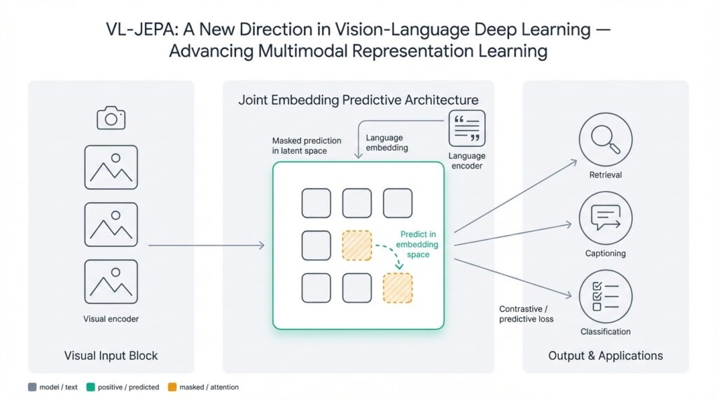
VL-JEPA rethinks how we learn joint image-text representations by predicting high-level targets in embedding space rather than forcing direct pixel- or token-level reconstruction. In practice this means we train a context encoder to produce a compact latent that predicts a target latent produced from another view or modality — so vision-language and multimodal representation learning become prediction problems in representation space. Building on that foundation, VL-JEPA shifts emphasis from pairwise matching to generative prediction, which often yields richer semantics for downstream tasks like retrieval, captioning, and few-shot transfer.
The core idea is straightforward: split the model into three roles — a context encoder that ingests an image region or text span, a target encoder that provides the prediction target (usually from a different view or a masked portion), and a lightweight predictor that maps context latents into the target latent space. Define your loss as a distance (L2, cosine, or a contrastive margin) between predicted and target embeddings. This setup avoids forcing modality-specific alignment at the raw-input level and instead enforces consistency of high-level features, which helps when you need representations that generalize across domain shifts or noisy captions.
How does VL-JEPA differ from traditional contrastive vision-language methods? Contrastive approaches like CLIP train by pulling matching image-text pairs together and pushing non-matching pairs apart, which optimizes relative similarity but can underemphasize intra-modal structure. VL-JEPA, by predicting a concrete embedding target, preserves richer topology inside each modality while still learning cross-modal mappings. For you as a practitioner, that often means embeddings that capture compositionality (object attributes, relations) and are easier to fine-tune for generative or localization tasks.
Architectural choices matter: use a transformer or convolutional backbone for the vision encoder and a transformer for text, then project both into a shared latent space via small MLP heads. The target encoder can be a momentum (teacher) network updated with exponential moving averages to stabilize targets, a technique borrowed from self-supervised learning that reduces collapse without negative samples. Optionally mask image patches or text spans before encoding targets to force the predictor to infer missing semantics; this creates a form of cross-modal masked modeling that improves robustness to occlusion and noisy captions.
To make this tangible, here is a compact pseudocode sketch of a VL-JEPA training step you can adapt to your codebase:
# x_img, x_text: augmentations or masked views
z_ctx = ContextEncoder(x_img)
z_tgt = TargetEncoder(x_text)  # momentum/EMA model
z_pred = Predictor(z_ctx)
loss = loss_fn(z_pred, stop_gradient(z_tgt))  # L2 or cosine
loss.backward(); optimizer.step()
update_momentum(TargetEncoder, ContextEncoder, tau=0.995)
That pattern emphasizes stable targets (stop_gradient) and a simple prediction objective. In experiments we run, choosing cosine similarity for loss and normalizing embeddings before prediction often leads to better transfer performance, while L2 losses can be more stable for continuous latent spaces. Also consider curriculum strategies: start with small masked ratios and increase masking as training progresses to avoid optimization collapse when models are uninitialized.
From a deployment perspective, VL-JEPA models are useful when you need compact multimodal encoders that can be fine-tuned for classification, retrieval, or generative conditioning without retraining large contrastive heads. For instance, use the shared latent as a conditioning input for a captioning decoder or as a retrieval key in a production search service; the prediction-trained latents tend to be more robust to caption noise and viewpoint changes. Taking this concept further, the next section will examine training recipes and hyperparameters that consistently produce stable, transferable VL-JEPA representations.
JEPA background and motivation
JEPA and its VL-JEPA adaptation answer a practical pain point we’ve all seen in multimodal systems: aligning images and text at the raw input level forces models to waste capacity on low-level details instead of learning the high-level semantics you actually care about. In the first few training hours, pixel- or token-level reconstruction and naive contrastive matching reward surface similarity—color histograms, stopwords, or image textures—rather than object relations and compositional meaning. By training the model to predict a high-level embedding target, JEPA (joint embedding predictive approach) directs learning toward representations that encode semantics useful for downstream multimodal representation tasks like retrieval, captioning, and conditioning generative decoders.
The idea has roots in predictive representation learning and masked modeling, but its motivation is distinct: preserve intra-modal structure while enabling cross-modal inference. Predictive methods such as contrastive predictive coding and masked autoencoding showed that forcing a model to predict missing information creates stronger, more transferable features than reconstructing raw inputs. JEPA inherits that insight and reframes cross-modal alignment as a prediction problem in latent space—so instead of pulling an image and its caption together or reconstructing pixels, you make the context encoder predict a target embedding produced from another view or masked span. This preserves modality-specific topology while still teaching the model to infer across modalities.
Why does predicting embeddings produce better transfer than matching pairs? The core reason is information bottlenecking: embeddings abstract away high-frequency noise and modality idiosyncrasies, so the predictor must capture relational and compositional features to succeed. When you optimize a distance in embedding space, gradients push the model to encode attributes that survive projection—object presence, attributes, interactions—rather than incidental background colors or common stopwords. Practically, that yields latents that generalize across caption noise, viewpoint changes, and domain shifts because the optimization objective focuses on semantically stable features instead of pixel fidelity.
Consider a concrete production scenario: an e-commerce visual search pipeline where product photos vary by lighting and text descriptions are noisy or abbreviated. If you train with contrastive loss alone, the model may overfit to consistent but irrelevant tokens (brand suffixes) or background patterns; a JEPA-style predictor instead learns to infer missing attributes (color, style, category) from a masked caption or alternate view, producing embeddings that align on product semantics rather than accidental cues. That makes downstream retrieval more robust and reduces manual engineering for normalization of noisy text.
So when should you pick JEPA over contrastive or reconstruction-based approaches? Ask what downstream tasks you prioritize. If your primary need is large-scale nearest-neighbor retrieval with millions of items and you can rely on strong negative mining, contrastive learning scales well. If you need transferable generative conditioning, compositional reasoning, or localization, JEPA is often the better choice because it enforces predictive structure inside the latent manifold. Also consider data quality: JEPA excels when captions are noisy or when you want robustness to occlusion and viewpoint shifts, because predicting targets forces the model to infer missing semantics rather than memorize pairwise similarity.
There are practical trade-offs to manage when you adopt this pattern. Preventing target collapse requires a stable target encoder (momentum/EMA or a slow-moving teacher), predictor capacity tuning, and embedding normalization; otherwise the predictor can trivially minimize loss by shrinking outputs. Curriculum masking—starting with low mask ratios and increasing them—helps optimization early on, and cosine objectives with normalized embeddings often improve transfer for multimodal representation. Monitor downstream probes (few-shot classifiers, retrieval mAP) during development rather than training loss alone, since embedding prediction can decouple training loss from semantic quality.
Building on this foundation, the next step is to translate these motivations into concrete training recipes and hyperparameter choices so you can get stable, transferable VL-JEPA representations in your codebase. We’ll next walk through optimizer settings, masking schedules, predictor architectures, and validation strategies that reflect the trade-offs described here.
Model architecture and modules
VL-JEPA reframes multimodal representation learning by splitting responsibilities across compact, well-defined modules, and our architecture choices determine whether the learned predictive latent actually captures compositional semantics. How do you design those modules so prediction in embedding space is stable, efficient, and transferable? We start from three principal roles you already saw in the overview—context encoder, target encoder, and predictor—and then make concrete architectural decisions: backbone choices, projection heads, normalization layers, and lightweight predictor topology that together form a robust joint embedding predictive approach (VL-JEPA) pipeline.
The context encoder is where input modality-specific structure is first converted into a dense representation, and you should pick its backbone to match the input scale and task. For images, use a Vision Transformer for long-range relational reasoning or a CNN/ConvNeXt variant if compute and latency are constrained; for text, a transformer with subword tokenization and rotary or learned positional encodings works well. Immediately after the backbone, add a small MLP projection head (two layers with GELU and a residual skip) to map modality-specific features into the shared latent dimension; this projection reduces cross-modal capacity mismatch and becomes the predictor’s input. Keep the context encoder’s output compact (512–2048 dims depending on downstream) to control predictor size and retrieval index cost.
The target encoder provides the stable embedding the context must predict, and its stability is central to preventing collapse. Implement it as a momentum/EMA teacher that mirrors the context architecture but uses slow parameter updates (tau in 0.995–0.999 range) and stop-gradient on its outputs. Optionally apply aggressive masking to the target input—masked image patches or removed text spans—so the predictor must infer missing content from context; this cross-view masking trains the model to fill gaps rather than memorize surface cues. Consider using separate projection heads for targets (slightly wider bottleneck) to encourage targets to encode richer semantics while keeping prediction manageable.
The predictor is intentionally lightweight but expressive enough to map context latents into the target manifold without trivial collapse. A 2–4 layer MLP with LayerNorm and residual connections often suffices for many use cases; for cross-modal structural prediction (e.g., predicting masked relations), a shallow transformer predictor can capture pairwise interactions in the latent. Tune predictor capacity carefully: under-parameterized predictors underfit and provide weak gradients, while over-parameterized ones can learn shortcuts that ignore meaningful structure. We prefer pre-normalizing the context latent before the predictor and using a final projection that enforces the target dimensionality.
Loss design and embedding normalization bind the architecture together and influence transfer. Use cosine similarity with unit-normalized embeddings for transfer-focused objectives, and use L2 when you expect continuous latent interpolation for generative conditioning. Implement stop-gradient on the target encoder and normalize both prediction and target vectors to unit norm before computing cosine loss; if you use contrastive margins, include a temperature parameter and sample negatives within batch or via a memory bank. To avoid target collapse, add small predictor weight decay, occasional target centering, or a variance-preserving regularizer on the target outputs.
Training-time modules and schedules are as important as topology: data augmentation, masking curriculum, and EMA scheduling all affect convergence. Start with modest mask ratios (10–20%) and warm the predictor for several epochs before raising masks to 40–50% if you aim for robust occlusion inference; gradually increase EMA tau as representations stabilize. Use multi-view sampling—two image augmentations and one masked caption, or vice versa—to provide richer prediction targets per batch, and prefer large batch sizes or effective large-batch optimization (LARS/AdamW with linear scaling) to stabilize the predictive objective.
At inference, decompose responsibilities to reduce runtime cost: you generally only need the context encoder and the shared projection head to produce the predictive latent used for retrieval or as conditioning input. The target encoder and heavy predictor are training-time scaffolding unless you explicitly require predicted targets for downstream tasks; for example, attach the learned latent to a lightweight captioning decoder or use it as a retrieval key in a vector DB. Building on this modular view lets us iterate on individual pieces—backbone, predictor, loss schedule—without retraining the entire system, which is why architecture and module choices matter for practical VL-JEPA deployments.
Training objectives and losses
VL-JEPA reframes learning as embedding prediction, and that reframing drives different choices for your training objective compared with standard contrastive or reconstruction losses. From the start, prioritize an objective that measures distance in latent space rather than pixel/token fidelity—cosine similarity on unit-normalized vectors and L2 (mean squared) distance are the two most common options, with contrastive margins as an optional hybrid when you need relative ranking. Building on the overview, we recommend front-loading embedding prediction and cosine similarity in early experiments because they bias the model toward semantic alignment across modalities and transfer-friendly representations.
The simplest objective is a direct prediction loss: compute z_pred = Predictor(z_ctx) and minimize distance(z_pred, stop_gradient(z_tgt)). This enforces that the context encoder must produce a latent that predicts the target encoder’s embedding, and you should always stop-gradient on the target to avoid collapse. Use cosine similarity when you care about directional alignment and downstream retrieval; choose L2 when you plan to use latents for continuous generative conditioning or interpolation. For some tasks, combining a cosine reconstruction term with a small contrastive margin (sampled negatives within-batch) gives the best of both worlds—stable prediction plus relative discrimination.
How do you choose between cosine similarity and L2 for embedding prediction? Cosine similarity with unit-normalized embeddings emphasizes angular relationships and often yields better retrieval and transfer performance, while L2 preserves scale and can be more stable for continuous latent manifolds used by generative decoders. If you use cosine, normalize both z_pred and z_tgt and optionally multiply the loss by a learnable temperature to control gradient magnitude. If you add contrastive components, include a temperature hyperparameter and ensure negative sampling is diverse—large effective batch sizes, memory banks, or asynchronous queues help the contrastive margin remain informative.
Preventing collapse and trivial solutions is the most important practical concern when optimizing prediction objectives. Implement a momentum (EMA) target encoder and apply stop-gradient to its outputs; set tau in a warm-up window (e.g., 0.995–0.999) and consider increasing tau as training stabilizes. Regularize the predictor with modest weight decay, add LayerNorm or residual connections to avoid shortcut learning, and keep predictor capacity balanced—too small and gradients vanish, too large and it memorizes mapping without improving context representations. We also find that applying a small variance-preserving regularizer or occasionally centering target outputs (subtracting running mean) keeps the target distribution well-conditioned.
Training schedules and masking curriculum directly interact with loss behavior and convergence. Start with light masking (10–20%) and a predictor warm-up for several epochs, then raise mask ratios to 40–50% if you want robust occlusion inference; this reduces early optimization pressure and avoids degenerate minima. Use AdamW with linear warmup and cosine decay or scaled LR rules for large batches; effective large-batch training stabilizes embedding prediction objectives and enables better negative mining when you include contrastive terms. In an e-commerce visual-search example, increasing mask ratios while using cosine loss and an EMA teacher produced embeddings that matched product attributes across varied photos and noisy captions, improving retrieval mAP in production.
Finally, monitor the right signals during development: track embedding-level metrics (cosine alignment, variance, norm statistics), downstream probes (few-shot classification, retrieval mAP), and qualitative checks (nearest-neighbor attribute consistency). Loss alone can be misleading because embedding prediction decouples training loss from semantic utility; therefore we recommend early checkpoints evaluated on small retrieval and captioning probes. Taking these practices together will make your embedding prediction objective stable and transferable—building a solid foundation before we tune optimizer settings, masking schedules, and predictor topology in the next section.
Selective decoding and inference
Selective decoding is how you decide which parts of a VL-JEPA pipeline to run at inference time so you meet latency, cost, and quality targets. Building on the predictive-embedding foundation we covered earlier, the core idea is to avoid executing every training-time module (momentum target, heavy predictor, masked decoders) for every request; instead, we choose a minimal compute path that preserves the semantics you need. This matters for multimodal representation systems because small reductions in per-query cost compound across millions of requests, and because inference choices change the practical signal the downstream model receives. How do you balance speed and semantic fidelity in production?
Start by categorizing inference workloads by objective: retrieval, reranking, generation, or localized prediction. For high-throughput nearest-neighbor retrieval, run only the context encoder plus projection head to produce the shared latent, normalize it (cosine-friendly), and use an ANN index—this keeps latency and memory low while preserving the VL-JEPA-trained semantics. For higher-precision tasks like captioning or relation extraction, add a shallow predictor or a lightweight decoder conditioned on the context latent; this extra step recovers masked or cross-modal semantics learned during training without invoking the full teacher model. Choosing which modules to execute should be guided by the downstream utility you measured during development (retrieval mAP, caption BLEU/ROUGE proxies, or attribute classification accuracy).
A practical, common pattern is two-stage selective decoding: first stage is a cheap, dense-embedding pass for retrieval; second stage selectively decodes only the top-K results with heavier models. Implement this by computing z_ctx = ContextEncoder(x) and storing z_ctx in your vector DB. At query time, run an ANN search to get candidates, then run z_pred = Predictor(z_ctx_query) or a small cross-attention reranker across image-text pairs only for the top-K. Example pseudocode captures this flow succinctly:
# stage 1: fast vector retrieval
z_q = ContextEncoder(query)
candidates = ANN.search(z_q, top_k=100)

# stage 2: selective decoding for high-precision ranking
rank_scores = [Reranker(z_q, z_c) for z_c in candidates]
final = sort_by(rank_scores)[:10]
This selective approach preserves the VL-JEPA benefit—prediction-trained latents that encode compositional attributes—while limiting heavy compute to a small subset of items. For caption generation, condition a small autoregressive decoder on the shared latent rather than running the full target encoder; that keeps generated text grounded in the prediction-trained manifold and avoids the cost of running an EMA teacher at inference. When you need calibrated probabilities or token-level uncertainty, append a light posterior head to the decoder; otherwise prefer deterministic decoding from the compact latent for repeatable, low-latency outputs.
Operational optimizations further reduce cost without sacrificing semantics. Cache and shard precomputed latents for content that changes infrequently, and combine that with product quantization or OPQ to shrink the ANN storage budget. Use asymmetric compute: quantize the retrieval index aggressively (e.g., 8-bit or PQ) while keeping the reranker in float16 or float32. Distill a heavier predictor into a small MLP for on-device inference, and add an early-exit mechanism in deeper predictors so low-complexity inputs bypass full computation. These techniques let you trade a small accuracy delta for substantial throughput gains in production multimodal representation services.
Deciding which selective decoding strategy to use depends on your SLOs, traffic profile, and the downstream probe metrics you care about. Measure retrieval mAP, few-shot classification accuracy, and generation quality under each candidate inference path; prefer the simplest pipeline that meets those metrics. Building on the training and architecture choices we discussed earlier, selective inference lets us deliver the semantic richness of VL-JEPA representations in a practical, cost-effective way—next we’ll translate those deployment patterns into concrete training recipes and validation checks that ensure the inference-time shortcuts preserve the representation quality you rely on.
Implementation code walkthrough
Building on the conceptual foundation we covered earlier, this walkthrough shows how to turn VL-JEPA’s embedding prediction idea into reproducible code you can run and iterate on. We start from the modules you already know—the context encoder, the target (EMA) encoder, and a lightweight predictor—but focus on concrete implementation details that influence stability and transfer in multimodal representation learning. You’ll see practical choices for batching, masking, normalization, and checkpointing that matter when moving from paper pseudocode to a production-friendly training loop.
A robust data pipeline is the first implementation challenge you’ll face. Prepare multi-view batches that mix two image augmentations with one masked caption or vice versa so each context-target pair forces cross-view inference; for text use span masking of 15–40% depending on caption length, and for images mask patches with block-based sampling instead of IID pixel drop to preserve spatial relations. Use deterministic tokenization and cache tokenized captions for large corpora to reduce I/O; enable mixed-precision and gradient accumulation if your effective batch size must scale beyond GPU memory. These choices directly affect the embedding distribution and the quality of downstream retrieval and few-shot probes.
Now let’s walk through the core training update you’ll implement in PyTorch-style pseudocode and why each step exists. The key operations are: encode context, encode target with stop-gradient, predict, compute loss (cosine or L2), backprop, and update the EMA teacher. The snippet below shows the minimal loop we use in experiments:
# x_img, x_text: sampled views
z_ctx = context_encoder(x_img).proj()          # normalize prior to predictor
z_tgt = target_encoder(x_text).proj().detach() # stop-gradient on teacher
z_pred = predictor(z_ctx)
loss = cosine_loss(F.normalize(z_pred), F.normalize(z_tgt))
loss.backward(); optimizer.step(); optimizer.zero_grad()
# EMA update: tau typically 0.995-0.999, linear warmup of tau useful
for p_t, p_s in zip(target_encoder.parameters(), context_encoder.parameters()):
    p_t.data = tau * p_t.data + (1 - tau) * p_s.data
Pay attention to where you normalize and where you detach. Pre-normalizing the context latent before the predictor and normalizing outputs before the cosine loss stabilize gradients and improve retrieval transfer. We prefer AdamW with weight decay on the predictor but lighter decay on the encoder to preserve representation capacity; use cosine LR decay with a short linear warmup and gradient clipping (1.0) to avoid optimizer spikes. If you use L2 loss instead of cosine because you plan to use latents for generative conditioning, skip unit normalization and monitor embedding norm statistics closely.
How do you detect and debug collapse or poor predictors in practice? Instrument several lightweight probes during training: embedding variance per-dimension, mean norm, nearest-neighbor attribute consistency on a small held-out set, and a tiny retrieval mAP computed every epoch. If variance collapses toward zero or nearest neighbors stop reflecting semantic attributes, increase EMA tau, add a variance-preserving regularizer (e.g., small scale normalization loss), or reduce predictor capacity—over-parameterized predictors sometimes learn trivial mappings that hurt context learning. We also recommend checkpointing both encoder and predictor states frequently and running downstream few-shot evaluations to ensure training loss correlates with semantic utility.
Finally, implement inference exports and selective decoding early so you don’t rework pipelines later. At serving time you typically only need the context encoder and projection head saved as a single traced model (ONNX/torchscript) with float16 support; keep the predictor and EMA teacher for optional reranking or for distillation into a tiny on-device MLP. Quantize or product-quantize stored vectors in your ANN index and shard encodings for batch queries to meet SLOs. Taking these implementation steps together lets you move from VL-JEPA theory to a stable, deployable multimodal representation system—and next we’ll tune hyperparameters and masking schedules based on the probes you’ve added here.