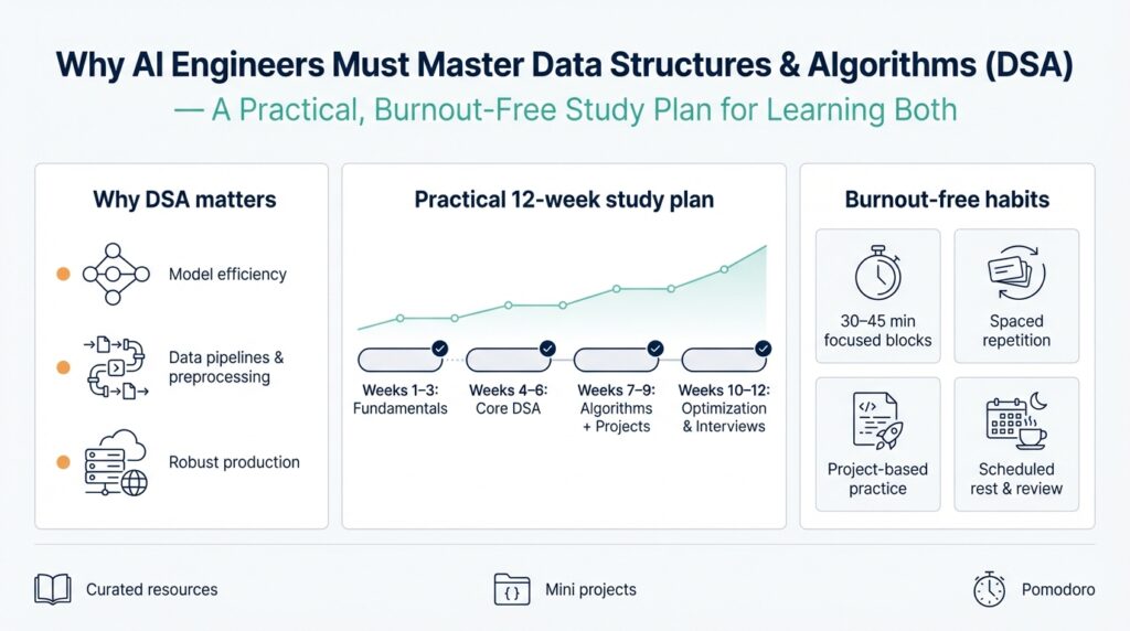
Why DSA Matters for AI
Building on this foundation, data structures and algorithms matter for AI because they determine whether your model is usable in production or remains an expensive research artifact. When you design training pipelines, retrieval systems, or real-time inference, choices about data organization and algorithmic strategy directly control latency, throughput, and cost. For AI engineers, mastering data structures and algorithms gives you predictable performance trade-offs instead of guessing at bottlenecks. We’ll use this understanding to prioritize optimizations that actually move metrics rather than wasting cycles on micro-tuning model weights.
Performance at scale is not a nicety—it’s a constraint you must engineer around. Algorithmic efficiency (how time and memory grow with input size) defines the difference between an offline experiment and a service-level objective you can guarantee. For example, understanding amortized time complexity—how the average cost per operation behaves over sequences of operations—lets you pick a buffer, queue, or index structure that minimizes tail latency. In production pipelines, an O(n log n) preprocessing step can be acceptable once, but an O(n^2) step in a per-request hot path will create outages; we need to design around that.
Concrete architectures show these trade-offs. Consider nearest-neighbor search for vector embeddings: exact KD-tree search works well for low-dimensional vectors and gives deterministic correctness, while approximate methods like HNSW or product-quantization trade some recall for orders-of-magnitude lower latency and smaller memory footprint. When you choose an index, ask whether your workload tolerates occasional false negatives and whether latency or recall drives business value. In code, this translates to using a priority queue-backed beam search for constrained decoding or swapping to an ANN index for large-scale semantic search; the implementation pattern determines whether queries hit SSDs, RAM, or GPU memory.
Data structures also shape reliability and observability. Use Bloom filters (a probabilistic membership structure) to cheaply gate expensive downstream work such as expensive feature computation or model scoring; the controlled false-positive rate is a tunable knob. Hash maps with careful sharding and lock-free designs reduce contention on high-throughput feature servers. For streaming features, circular buffers and windowed aggregates let you compute statistics with bounded memory; these are the kinds of choices that prevent memory leaks and OOMs during traffic spikes in production.
Beyond micro-optimizations, algorithmic thinking changes how you approach model design and debugging. How do you choose between exact and approximate, or between batch and streaming? You profile the hot path, quantify cost in CPU/GPU seconds and tail latency percentiles, and then apply a targeted algorithmic improvement—replace an O(n) scan with an indexed lookup, move from synchronous to eventual consistency, or precompute embeddings. Graph neural networks are a telling example: naive neighborhood expansion is O(n^2) and will explode; sampled neighbor algorithms and sparse matrix primitives reduce complexity and enable training on billion-edge graphs.
Because these choices interact with your infrastructure and product constraints, learning DSA is not an academic exercise—it’s practical engineering. Building on what we covered earlier, the next section will map these principles into a step-by-step, burnout-aware study plan that helps you practice the right patterns (indexing, streaming, caching, approximate algorithms) on real workloads. That plan will show how to turn algorithmic insights into measurable production improvements so you can ship faster and maintain confidence under load.
Essential Data Structures Overview
Building on this foundation, the concrete toolbox you need as an AI engineer centers on a small set of proven data structures whose trade-offs show up again and again in model pipelines, feature stores, and real-time inference. In the next paragraphs we’ll define those structures, explain when to pick each one, and show practical patterns—so you can move from conceptual gains to measurable latency, memory, and cost improvements. We focus on algorithmic efficiency and predictable performance because those are the knobs you’ll tune in production.
Start with arrays and contiguous buffers: they give O(1) indexed access and compact memory layout that modern CPUs and GPUs exploit. Use arrays (or tensors) for dense feature representations and minibatch operations where throughput matters; prefer contiguous layouts to reduce cache misses and avoid strided accesses that degrade vectorized computation. When you need a rolling window for streaming features or online statistics, swap to a circular buffer (ring buffer) to maintain fixed memory while supporting amortized O(1) push/pop—this prevents unbounded memory growth during traffic spikes.
Hash tables (maps) are the go-to for constant-time average lookups and are indispensable for feature servers, vocabulary-to-id mappings, and caching precomputed embeddings. Choose open-addressing or chained hash maps depending on load factor and memory fragmentation patterns; for high-throughput feature stores, shard the hash map across threads or use lock-free variants to avoid contention. Also consider LRU or segmented caches on top of hash maps when evicting stale embeddings reduces downstream compute.
Heaps and priority queues provide efficient top-k and scheduling semantics: they implement logarithmic insert/delete-min operations and are perfect for beam search, online top-k monitoring, and delayed-job scheduling. For example, maintain a fixed-size min-heap of size k to implement streaming top-k with O(log k) updates per insert. On the implementation side, use binary heaps for simplicity or pairing/fibonacci heaps when you need faster decrease-key in complex graph algorithms.
Trees—binary search trees, balanced trees (AVL/Red-Black), and prefix trees (tries)—model ordered data and hierarchical keys. Use balanced trees when you need ordered iteration with guaranteed logarithmic operations, for example in range queries over timestamped model metrics. Tries shine for prefix-heavy lookups such as tokenization and autocompletion; they trade memory for deterministic lookup times and can be compressed (radix trie) to reduce footprint in vocabulary-heavy NLP systems.
Graphs and sparse matrices are must-haves for relational and GNN workloads: represent relationships explicitly with adjacency lists for sparse graphs, and prefer CSR/CSC (compressed sparse row/column) formats for linear algebra that interfaces with optimized sparse BLAS kernels. Sampled neighbor algorithms and sparse multiplication reduce the O(n^2) explosion when you expand neighborhoods; in practice, implement neighbor sampling with reservoir samplers or alias tables to keep training throughput predictable.
Probabilistic and approximate structures give huge wins when exactness is unnecessary: Bloom filters, Count-Min Sketch, and HyperLogLog let you trade a bounded error for orders-of-magnitude savings in memory. Use a Bloom filter to gate expensive model scoring (cheap membership test with tunable false-positive rate) and Count-Min Sketch for approximate frequency counts on high-cardinality features. For large-scale semantic search, pair these structures with ANN indexes (HNSW, PQ) to reduce memory and query cost while retaining acceptable recall.
Throughout these choices, ask practical questions: How does operation complexity map to your per-request budget? Can you tolerate occasional approximation to save RAM or reduce tail latency? The next section will convert these design patterns into hands-on exercises and small, production-like projects so you can practice implementing and measuring these data structures under real workloads. By grounding learning in deployment constraints, we prioritize the structures and algorithms that move SLOs rather than theoretical coverage alone.
Core Algorithms for AI
Building on this foundation, the algorithms you choose are the levers that convert model research into reliable, cost-effective systems; mastering core algorithmic families lets you predict how latency, memory, and cost will scale under real traffic. In this section we focus on the algorithmic patterns that repeatedly appear in production AI: search and indexing, numerical linear algebra, graph and sampling algorithms, streaming/online routines, and practical scheduling/optimization heuristics. How do you decide which approach belongs in your hot path versus an offline precompute? We’ll answer that with concrete patterns and decision criteria you can apply to real pipelines.
Search and indexing algorithms shape interactive features like semantic search and recommendation. Exact nearest-neighbor search (KD-trees, VP-trees) gives deterministic recall but degrades with high dimension; approximate nearest neighbor (ANN) algorithms such as HNSW and product quantization trade a bounded loss in recall for orders-of-magnitude latency and memory improvements. Use ANN when tail latency or RAM footprint is the gating factor and your application can tolerate occasional misses; prefer exact indexes for low-dimensional or strongly consistency-driven workloads. In practice, implement a tiered index: a memory-backed ANN for low-latency reads and a slower exact fallback for low-recall cases, and measure end-to-end recall/latency against business SLOs.
Numerical linear algebra is the workhorse behind embeddings, PCA, and low-rank compression. Blocked matrix multiplication, fused kernels, and using vendor BLAS/LAPACK primitives reduce constant factors—so an O(n^3) operation can be feasible for moderate n when implemented with optimized kernels. For dimensionality reduction at scale, randomized SVD and incremental PCA give near-identical quality with far less memory than the full SVD; store dense factors in contiguous arrays to exploit cache and GPU bandwidth. When you operate on sparse data, prefer CSR/CSC formats and sparse BLAS so you avoid materializing dense intermediates that explode memory and ruin throughput.
Graph and combinatorial algorithms appear in GNNs, sessionization, and dependency analysis. Naive neighbor expansion is explosive; sampled neighbor strategies (e.g., uniform or importance sampling) keep per-node work bounded and preserve training throughput. Use Dijkstra or A* for constrained path-finding problems where edge weights matter, and reservoir sampling or the alias method when you need unbiased subsamples from streaming neighbors. Implement neighbor sampling as a composable primitive so you can swap sampling distributions without changing the outer training loop.
Streaming and sketching algorithms let you maintain useful statistics with bounded memory and predictable cost. Count-Min Sketch provides heavy-hitter approximations for high-cardinality features, and approximate quantile algorithms (e.g., t-digest or P^2) give latency-aware percentiles without storing full windows. For bounded-memory top-k, maintain a fixed-size min-heap and evict the minimum on overflow—this gives O(log k) updates per record and deterministic memory use. These approximate structures are powerful tools when you must trade a tunable error for consistent algorithmic efficiency at scale.
Scheduling, batching, and search heuristics are the operational algorithms that reduce effective cost per inference. Dynamic batching groups requests by input shape or model signature and flushes on max-batch or latency window; implement as a single-producer queue with a timer and a batch-merge function to keep tail latency predictable. For sequence generation, decide between greedy, beam search, or constrained decoding based on quality-latency trade-offs—beam search increases computation roughly by the beam factor, so encode that into your SLO math. These operational algorithms often yield larger dollar-and-latency wins than micro-optimizing model internals.
To apply these patterns, profile with controlled scaling experiments: vary input cardinality, dimension, and concurrency while recording tail latency, memory, and cost. Quantify algorithmic efficiency in practice, not just Big-O: measure per-item CPU/GPU seconds and tail percentiles, then choose whether to replace exact work with ANN, sampling, or sketching. Taking this approach lets us prioritize the algorithmic changes that move production SLOs; the next step is hands-on exercises that help you implement, benchmark, and iterate on these core algorithms under realistic workloads.
Applying DSA to ML Pipelines
Building on this foundation, the hardest practical gap for teams is turning abstract data structures and algorithms into concrete, testable parts of an ML pipeline rather than leaving them as ad-hoc knobs you tweak after things break. You need to treat data structures and algorithms as first-class design decisions at each pipeline stage: ingestion, feature computation, indexing, and serving. When you do that, you convert unpredictable tail latency and runaway costs into measurable engineering choices you can optimize against SLOs and budgets. This section shows how to map those choices to code patterns and operational experiments you can run today.
Start by mapping pipeline stages to algorithmic families so you pick the right trade-offs early. For ingestion and streaming, favor bounded-memory structures—circular buffers (ring buffers) for fixed-size windows and reservoir sampling for unbiased stream subsamples—because they make latency and memory predictable. For feature stores and lookups, use sharded hash maps or lock-free maps to avoid contention at high QPS; add a small LRU cache layer when recomputing embeddings is costly. For indexing and retrieval, design a tiered index where an in-memory ANN (approximate nearest neighbor) handles most queries and an exact on-disk fallback handles low-recall cases; that pattern gives you a measured balance between latency, recall, and cost.
Make streaming feature computation concrete by composing small, predictable primitives rather than monolithic jobs. For example, implement a rolling quantile with a fixed-size ring buffer and a t-digest sketch for long tails so you never store unlimited history. Use a Count-Min Sketch for high-cardinality frequency estimates to gate expensive downstream computation: perform a sketch lookup, and only if the frequency exceeds a threshold do you compute heavy features. In code this looks like a producer pushing events into a ring buffer while a worker thread updates a Count-Min Sketch and a compact digest; the result is bounded memory, amortized O(1) updates, and an operational knob (sketch error/size) you can tune.
When you design retrieval, ask a simple question: When should you swap to ANN instead of exact search? Use ANN (HNSW, product quantization) when dimensionality and corpus size make exact search exceed your latency or RAM budget and when occasional recall loss is acceptable. Quantify that decision by running a tiered experiment: measure 99th-percentile latency and end-to-end recall (business metric) for in-memory ANN, then enable an exact fallback for low-confidence queries. Pair the index with a Bloom filter to cheaply reject cold-start or non-existent IDs before hitting the index; Bloom filters trade a tunable false-positive rate for huge savings in downstream work and are simple to operationalize.
Operational algorithms often yield the largest wins, so design them into your hot paths. Implement dynamic batching as a single-producer queue plus a timer: flush either when batch size reaches N or when latency exceeds T, and merge compatible requests to maximize GPU throughput without violating tail latency SLOs. Use a fixed-size min-heap to maintain streaming top-k metrics with O(log k) updates, and implement backpressure by rejecting or degrading non-critical work when queue depth crosses thresholds. These patterns convert algorithmic complexity into clear SLO math—CPU/GPU-seconds per request, memory per connection, and expected tail latency given concurrency.
Finally, validate every choice with controlled profiling and synthetic scaling so algorithmic efficiency becomes measurable, not assumed. Run experiments that vary input cardinality, vector dimensionality, and concurrency while recording latency percentiles, memory use, and recall; instrument hot paths with microbenchmarks that report per-item CPU/GPU seconds. How do you know an optimization helped? If it reduces 99th-percentile latency or cost-per-query without unacceptable recall loss, it passed. Taking this disciplined approach lets us convert theoretical advantages into reliable production improvements and prepares us to practice these patterns in the hands-on study plan that follows.
Burnout-Free Study Schedule
Building on this foundation, create a study schedule that treats data structures and algorithms (DSA) as practical engineering skills you’ll apply to real pipelines, not abstract exam topics. Start by committing small, focused blocks for active practice—25–50 minute coding sessions with 5–10 minute recovery breaks—so you maintain cognitive energy for problem solving and system design. Schedule two weekly deep sessions (90–120 minutes) for project work where you integrate a data structure into a mini-pipeline (for example, a ring buffer feeding a streaming aggregator or a Count–Min Sketch gating expensive feature computation). Treat the schedule as an experiment: measure mental load, throughput of learning, and whether you can implement, test, and benchmark within each session.
Set clear learning outcomes for each week so you make measurable progress on data structures and algorithms rather than accumulating vague exposure. For every week, pick one structure (hash tables, heaps, tries, ANN indexes) and one algorithmic pattern (sampling, batching, neighbor sampling, dynamic batching) and define a small acceptance test: latency under N concurrent requests, memory under M megabytes, and a recall or accuracy threshold when relevant. Working toward concrete SLO-style goals aligns your practice with production reasoning we discussed earlier; it also provides objective stopping criteria so you avoid sunk-time perfectionism. When you reach the acceptance test, write a short readme that describes trade-offs, complexity, and the tests you ran.
How do you structure practice to avoid burnout while still building depth? Alternate focused implementation days with light synthesis days. On implementation days you code and benchmark: implement an open-addressing hash map variant, a fixed-size min-heap top-k, or a small HNSW-like ANN prototype and measure 95th/99th percentile latency with increasing load. On synthesis days you review trade-offs, summarize microbenchmarks, and convert observations into one-line operational rules (for example, “use ring buffer + t-digest for rolling quantiles when per-request memory must be bounded”). This cadence preserves progress without demanding marathon sessions and gives cognitive rest between high-effort coding and reflective consolidation.
Anchor learning in short projects that mirror production constraints so you practice decision-making, not puzzle solving. Build a tiny retrieval service that uses an in-memory ANN for most queries and an exact on-disk fallback; instrument it to record end-to-end latency, recall, and RAM usage. Or create a streaming feature worker that ingests events into a circular buffer, updates a Count–Min Sketch, and only materializes heavy features when the sketch indicates high frequency. These projects force you to apply amortized complexity thinking, eviction strategies, and operational algorithms like dynamic batching and backpressure—patterns that move SLOs in real systems.
Measure progress like an engineer: log metrics, run controlled scaling tests, and iterate on knobs. Use synthetic workloads to vary cardinality, vector dimension, and concurrency while recording CPU/GPU seconds per item and tail latency percentiles; compare those numbers to your acceptance tests. Keep a short change log where each entry records the hypothesis, the change (data structure or algorithm), and the quantified result—this not only reinforces learning but creates a cumulative reference you can revisit when debugging production incidents. If a change reduces 99th-percentile latency or cost-per-query without unacceptable functional loss, mark it as a successful pattern.
Finally, protect sustainability by planning for rhythm and review rather than continuous cram sessions. Reserve one weekly hour for knowledge consolidation: rewrite a failing implementation, refactor for clarity, or port a prototype into a testable library you can reuse across projects. Taking this approach helps you internalize data structures and algorithms as engineering habits—choices you’ll make by default when designing ingestion, indexing, or serving layers—so we can move from isolated exercises to reliably shipping efficient, maintainable AI systems.
Practice Platforms and Habits
Building on this foundation, the most productive way to learn DSA and make it stick is to treat practice as engineering work rather than exam prep. You should front-load focused coding practice that maps to real pipeline problems—implement a ring buffer, a Count–Min Sketch, or a tiny ANN index—not rote puzzle solving. How do you structure practice so that lessons transfer to production? We’ll show concrete platform choices and daily habits that turn algorithmic concepts into measurable system improvements while protecting your cognitive bandwidth.
Choose platforms that match the learning outcome you need. Use algorithmic problem sites (LeetCode, Codeforces, AtCoder) to sharpen asymptotic reasoning, complexity analysis, and fast prototyping of core routines like heaps, union-find, and trie operations. Use project-oriented platforms (GitHub, Kaggle, private sandboxes) to build small services that exercise design decisions: sharded hash maps for feature stores, a producer-consumer queue for dynamic batching, or a memory-backed ANN with an on-disk exact fallback. Match the platform to the task: contest sites for micro-skills, repos and notebooks for system-level patterns.
Structure your time with micro-sessions and two weekly deep sessions so practice scales without burning you out. Reserve 25–50 minute focused blocks for isolated problems (implement a min-heap top-k or a reservoir sampler) and schedule two 90–120 minute blocks for integrative work where you combine structures into a mini-pipeline. Alternate coding days with synthesis days: after an implementation session, spend a lighter session writing benchmarks, documenting complexity, and translating findings into one-line operational rules you can reuse in production.
Anchor every learning task in a tiny, production-like acceptance test so you practice decision-making as well as coding. Instead of ‘‘solve X problem,’’ define measurable goals: 99th-percentile latency under Y ms for N concurrent queries, RAM under M MB, and recall above R% for ANN experiments. Build a retrieval microservice that logs end-to-end latency and recall, or a streaming worker that maintains bounded memory with a ring buffer plus t-digest. These constraints force you to think in SLOs and trade-offs, not puzzle heuristics.
Instrument and benchmark everything you build; raw correctness is necessary but insufficient. Create synthetic workloads that vary cardinality, vector dimensionality, and concurrency while you capture 50/95/99th-percentile latencies, CPU/GPU-seconds per item, and memory footprints. Use lightweight microbenchmarks and timers in your code, and automate runs so you can compare changes objectively. When a tweak reduces 99th-percentile latency or cost-per-query without unacceptable recall loss, record the result and make it a reusable pattern.
Make review and collaboration part of the habit loop so you accelerate learning through feedback. Pair-program a tricky neighbor-sampling routine, run a code review focused on memory layout and cache friendliness, and keep a short changelog that records hypothesis, change, and measured outcome. Write a concise README for every mini-project explaining trade-offs (time complexity, memory use, and practical failure modes); that artifact is how knowledge passes from practice into your team’s baseline.
Taking these practices together creates a sustainable learning rhythm: focused problem sessions to sharpen core DSA skills, integrative projects to practice decision-making under SLOs, and disciplined measurement plus peer feedback to convert experiments into engineering patterns. With that rhythm in place, the next step is to translate one of those mini-projects into a repeatable lab exercise where you implement, benchmark, and iterate on a single production pattern.