Separating Hype from Reality
Building on this foundation, the first step is accepting that machine learning outcomes are narratives, not facts. The shiny demo you saw at a conference or in a research paper tells a story shaped by dataset choices, preprocessing, and tuned hyperparameters; it doesn’t automatically translate to your production workload. We need to separate marketing-grade anecdotes from engineering-grade evidence by demanding the same rigor we apply to any system: reproducibility, clear success metrics, and failure-mode analysis. Framing the problem this way prepares us to judge models on operational characteristics, not promises.
A reliable heuristic for cutting through hype is to ask targeted, testable questions about a claim before you invest resources. How do you tell whether a reported accuracy gain is substantive or noise? Insist on out-of-sample validation, multiple random seeds, and comparisons to strong non-ML baselines; these steps expose overfitting and fragile improvements. Also probe dataset provenance: was the data curated to make a model look good, or does it reflect your traffic and edge cases? Answering these questions quickly filters marketing from material advances and highlights real-world challenges such as dataset shift and label drift.
When evaluating a specific model, use a short practical checklist rather than intuition alone. Require reproducible training recipes and code, verify results on a holdout that mimics production, quantify inference latency and cost, and perform an error analysis focused on worst-case slices (not just average accuracy). For instance, an image classifier that performs well on clean validation images can still fail catastrophically on slightly different lighting or a new device camera—this is a common production trap. We also look for interpretability signals: are mistakes explainable, and can you trace them back to data issues or model capacity?
Turning a promising prototype into a deployed feature requires concrete gating criteria and an operational plan. Define the production success metric up front (conversion lift, false positive rate, mean time between failures) and set quantitative escalation thresholds. Deploy behind feature flags, run A/B tests that capture downstream business impact, and instrument real-time monitoring for data distribution changes and model drift. Create a retraining cadence and a rollback plan so you can respond when performance diverges; these engineering controls are where many projects labeled “AI-powered” fail in the real world.
Understanding trade-offs forces better decisions than chasing marginal accuracy gains. Consider latency, maintainability, observability, and regulatory constraints alongside model performance—sometimes a rule-based system or a simpler statistical model gives better end-user outcomes and lower operational risk. Weigh total cost of ownership: inference compute, annotation and labeling effort, and ongoing monitoring overhead. When compliance or explainability matters, prefer transparent models or hybrid architectures that combine deterministic business logic with ML where it demonstrably adds value.
Taking this concept further, you should treat every ML initiative as an engineering project with controlled experiments, acceptance criteria, and an operational lifecycle. As we discussed earlier, acknowledging practical limits helps you prioritize problems where machine learning is the right tool rather than the most attractive buzzword. If you adopt this mindset—demanding reproducibility, defining measurable success, and engineering for failure—you turn speculative hype into deployable capabilities that solve real-world challenges and produce predictable business value.
Fundamental Limits of ML
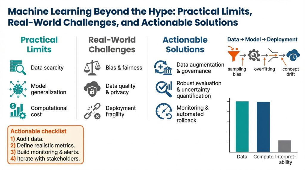
Building on this foundation, we need to confront the hard, structural constraints that determine what machine learning systems can — and cannot — reliably do in production. How do you know when a model’s failure is a fixable engineering bug versus a fundamental limit of the problem itself? Framing limits as statistical, computational, and adversarial helps you decide whether to invest in more data, better tooling, or a non-ML solution.
Some error is irreducible: even a perfect algorithm cannot beat noise inherent in the labels or the Bayes error for a task. Bayes error is the lowest possible error given the true conditional distribution P(y|x); when different labels are genuinely indistinguishable from the inputs you observe, no amount of model capacity will resolve that ambiguity. Label noise, weak supervision, and ambiguous specifications show up as persistent, correlated mistakes across models and random seeds — if repeated retraining and architecture sweeps don’t move those errors, you’re likely observing irreducible uncertainty.
Data distribution and sample complexity place practical ceilings on model generalization. Sample complexity is the number of labeled examples needed to reach a target performance; rare edge cases and long-tailed classes often require exponentially more examples than common cases. For instance, a medical imaging classifier for a 0.1% prevalence condition will need orders of magnitude more labeled examples or a different approach (transfer learning, active learning, or hierarchical rules) to achieve clinically useful sensitivity. When your learning curve flattens despite more compute and regularization, treat that as evidence the data distribution or label signal is the limiting factor.
Compute, optimization, and model expressivity impose computational limits that manifest differently from statistical limits. Nonconvex training, limited floating-point precision, and GPU memory caps can make certain architectures impractical at scale; states of the art sometimes trade inference latency and maintainability for marginal accuracy gains. We also see phenomena like double descent where increasing capacity first helps, then hurts, then helps again — which means brute-force scaling is not a universal strategy. The practical test is reproducible learning curves: measure performance versus data and capacity, profile optimizer behavior, and include cost-per-inference in your acceptance criteria before scaling out.
A separate class of limits comes from nonstationary and adversarial environments where the world actively changes or responds to your model. Concept drift, strategic behavior (fraudsters avoiding detection), and covariate shift can make yesterday’s model obsolete within weeks or days. In these settings, the fundamental limit is not a fixed accuracy ceiling but the ongoing mismatch between deployed behavior and the evolving distribution; we mitigate it with online learning, human-in-the-loop review for high-risk slices, and explicit game-theoretic thinking in feature design. Consider fraud detection: an ML model tuned to current attacker patterns will degrade as attackers adapt; detection systems must combine rules, anomaly detection, and rapid feedback loops rather than relying on a single static classifier.
Given these limits, the right engineering response is pragmatic: measure the dominant failure mode and choose controls that address it. If label noise or Bayes error dominates, invest in better labeling, richer feature collection, or change the product contract; if sample complexity is the blocker, prioritize active labeling and transfer learning; if compute or latency is the barrier, revisit model architecture and operational constraints; if adversaries drive drift, add online adaptation and human review. This diagnostic mindset helps you decide whether to continue iterating on models or to implement hybrid architectures and deterministic fallbacks — and it sets the stage for operational practices that keep models reliable over time.
Data Quality and Collection Issues
Building on this foundation, the technical reality of model performance often begins and ends with data quality and data collection choices you make up front. Poorly instrumented pipelines or ad hoc collection strategies create correlated failure modes that no amount of parameter tuning will fix, so the first engineering priority is treating data as a first-class asset. How do you detect label drift early, and how do you decide whether to invest in more labels versus changing the product contract? Framing these questions up front saves time and money when a prototype moves toward production.
The most common failure modes are predictable: label noise, sampling bias, sensor and ingestion errors, and silent schema changes in upstream systems. Label noise — inconsistent or ambiguous annotations — produces persistent, correlated errors across model families and random seeds, which is a telltale sign that the signal is in the labels rather than model capacity. Sampling bias and selection effects mean your training set will not reflect the production distribution; models that appear robust on curated validation sets fail on live traffic because corner cases are underrepresented. We find diagnosing the dominant data failure mode faster than iterating model architectures yields better ROI.
Annotation processes determine long-term label fidelity, so invest in clear guidelines and measurement of inter-annotator agreement before you scale labeling. Define explicit edge-case rules, run pilot annotation rounds, and compute agreement metrics such as Cohen’s kappa or Krippendorff’s alpha to quantify label noise; if kappa is low, don’t scale — fix the spec. Use active learning to prioritize human effort: surface high-uncertainty or high-impact examples for review, and bootstrap weak supervision patterns (labeling functions) only when you can measure their precision and coverage. These pragmatic controls reduce wasted labeling cost and improve downstream model calibration.
Dataset shift is not an abstract risk — it’s a root cause you can detect and mitigate with targeted sampling and domain-aware techniques. Distinguish covariate shift (P(x) changes) from label shift (P(y) changes) and selection bias; each requires different remedies such as importance weighting, domain adaptation, or targeted data acquisition for rare slices. For example, an image model trained on daytime photos will degrade on low-light phone captures — add stratified sampling for hardware and lighting conditions or deploy lightweight on-device augmentation to close that gap. When should you accept a deterministic fallback? If rare slices drive unacceptable risk and costs to label, a human or rule-based gate is often the right operational choice.
Operationalizing data quality requires continuous instrumentation rather than one-off checks: data contracts, schema validation, and streaming statistical tests must sit alongside feature stores and model metrics. Implement automated schema checks and incremental distribution tests (Population Stability Index, KL divergence, or streaming KS tests) for critical features, and run shadow inference to compare model outputs on live traffic without affecting users. Alert on meaningful shifts, route suspicious slices to human review, and log raw inputs to enable root-cause analysis; these practices make drift detectable within operational windows rather than after customer impact.
Put these ideas into an actionable short checklist you can adopt in week one: codify annotation guidelines and measure inter-annotator agreement, instrument ingestion with schema and provenance metadata, prioritize labeling with active learning, establish drift thresholds and shadow-mode validation, and define retraining triggers that combine statistical change with business-impact signals. Treat data collection as an engineering stream with SLAs, cost-per-label targets, and governance for sensitive features so that data quality becomes measurable and accountable. This operationalizes the diagnostic mindset from earlier sections and prepares you to decide whether more data, different labeling, or a non-ML fallback is the correct next step.
Model Robustness, Bias, and Safety
Model robustness, bias, and safety are not optional add-ons you bolt on after training — they determine whether a model survives real users, adversaries, and regulatory scrutiny. From day one you should treat robustness testing, bias audits, and safety controls as first-class engineering work that sits alongside data collection and deployment pipelines. We build on earlier points about dataset shift and operational controls: if you ignore these dimensions, high validation accuracy will look like a brittle promise when your model meets live traffic.
Start with a crisp definition: robustness means predictable performance under realistic perturbations and distributional shifts; bias means systematic errors that disadvantage particular groups or outcomes; safety means the system fails in ways that minimize harm and remain auditable. Adversarial examples — small, often imperceptible input changes crafted to break a model — are one extreme of non-robust behavior, while covariate shift and label drift are the everyday sources of performance degradation we discussed earlier. For example, an image classifier trained on studio photos that drops sharply on low-light phone images is a robustness failure rooted in sampling bias and inadequate augmentation.
You can operationalize robustness with targeted stress tests and uncertainty-aware inference. Run synthetic perturbation suites (noise, blur, color shifts, compression), adversarial attack simulations (fast gradient sign method, PGD), and domain-aware holdouts that reflect new devices or locales. Add a simple reject-on-uncertainty rule at inference to avoid confident mistakes: use entropy or max-softmax and a calibrated threshold — e.g., if max_softmax < 0.6 then route to human review. Small techniques—temperature scaling for calibration, ensembles for variance reduction, and test-time augmentation—often yield bigger safety wins than marginal accuracy gains from larger models.
Addressing bias starts with auditable datasets and slice-based evaluation. Ask: how do errors distribute across demographics, geographies, and edge conditions? Compute per-group calibration, false positive/negative rates, and worst-group accuracy rather than only global metrics. Remedial patterns include targeted data collection for underrepresented slices, reweighting or constrained optimization during training (e.g., equalized odds constraints), and counterfactual data augmentation to break spurious correlations. When labeling is ambiguous, codify annotation rules and measure inter-annotator agreement before scaling; unclear specs are the largest source of downstream bias.
Safety is broader than fairness: it’s about preventing and containing harm when models interact with humans and other systems. Define failure modes you care about (privacy leaks, unsafe recommendations, denial-of-service via model exploitation) and implement deterministic guards and escalation paths. For high-risk decisions, combine ML outputs with rule-based checks and human-in-the-loop approval gates; log raw inputs and decisions to enable post-hoc audits and incident analysis. Maintain a safety checklist that pairs statistical triggers (drift, calibration loss) with business signals (conversion drops, complaint spikes) to drive automated rollbacks.
How do you measure whether a model is robust across subpopulations? Use slice-based monitoring, holdout groups that mimic deployment heterogeneity, and an error budget tied to business impact: set a strict worst-case accuracy threshold for sensitive slices and alert when it trips. Instrument drift detectors per feature and per slice (population stability, KL divergence, or streaming KS tests), and prioritize retraining or human review based on impact-ranked alerts rather than raw statistical change alone. These controls connect directly to the production gating and rollback plans we recommended earlier.
Treat robustness, bias mitigation, and safety as continuous engineering practices, not one-time audits. Bake tests into CI, run shadow inference on live traffic, and make remediation cheap: automated labeling queues for failed slices, feature flags for quick rollbacks, and routine fairness and calibration reports. By integrating these controls into your model lifecycle we reduce surprise failures, improve trust, and make informed decisions about when to scale, retrain, or replace ML with deterministic fallbacks — which is the practical objective behind investing in robustness, bias, and safety up front.
Deployment, Scaling, and Cost Tradeoffs
Building on this foundation, the real engineering work begins when you turn a prototype into a reliably operating feature under real traffic—where deployment, scaling, and cost shape design decisions as much as model architecture. You’ll face hard tradeoffs between latency, throughput, and inference cost from day one, and those tradeoffs determine whether a model is feasible operationally, not just academically. How do you decide when to trade accuracy for latency or cost? The answer comes from quantifying SLOs, user impact, and total cost of ownership, then letting those constraints drive implementation choices.
Start by framing the operational objective in concrete terms: define per-request latency SLOs, throughput needs, and an acceptable cost-per-inference ceiling. If your product requires sub-50ms responses in the critical path, that constraint forces different options than offline batch scoring or background enrichment. For edge devices, on-device quantized models reduce network and inference cost at the expense of some accuracy; for high-volume backend services, batching, model distillation, or asynchronous workflows can lower cost while preserving user-facing fidelity. We find that stating the business-impact metric up front eliminates lengthy architecture debates.
Optimize inference before you horizontally scale. Techniques like quantization (lower-precision arithmetic), pruning (sparse weights), and distillation (training a smaller student network from a large teacher) materially reduce latency and inference cost without necessarily changing your data pipeline. In practice, try a small ablation: measure throughput and tail latency for float32 baseline, int8 quantized model, and a distilled student at comparable accuracy. Use micro-batching to increase GPU utilization for high-throughput services, and switch to single-request async handlers when tail latency matters. A short benchmark harness that measures p50/p95/p99 latency and cost-per-1M-requests will reveal whether optimization or scaling is the cheaper path.
Choose orchestration patterns that match load characteristics and your risk tolerance. Container orchestration and managed inference platforms simplify rollout and autoscaling, but they introduce node-management cost and scheduling overhead—especially with GPUs. Configure horizontal pod autoscalers for request-based metrics and use node pools to isolate expensive GPU instances; for bursty traffic, prefer serverless or spot-backed workers with warm pools to reduce idle GPU cost. Orchestration tools let you separate control-plane complexity from model serving, but we recommend small, measurable experiments: one model per service, a canary rollout, and observability hooks before you expand to many models.
Modeling cost needs to include more than compute: factor in storage, data transfer, labeling, and monitoring. A simple cost model helps decisions: monthly_cost ≈ (requests × cost_per_inference) + (training_runs × training_cost) + monitoring_and_labeling. When labeling rare slices is expensive, hybrid architectures—rules or human-in-the-loop for high-risk cases—often beat brute-force scaling. We’ve saved orders of magnitude by routing 99% of benign traffic to a cheap model and isolating expensive, high-risk inference to a small, audited pipeline.
Operational monitoring and safety instrumentation are cost centers that buy reliability. Shadow inference, per-slice drift detectors, and calibration checks increase observability cost but catch regressions before users see them. Decide which slices require continuous monitoring and which can be sampled; use escalation thresholds tied to business impact, not purely statistical drift, to avoid alert fatigue. Remember: the cheapest failure is the one you never let reach production because you detected and remediated it in shadow.
Make acceptance criteria and rollback plans explicit so you can scale with confidence. Treat scaling decisions as experiments: measure cost-per-accuracy point, start small with feature flags and canaries, and define an operational budget for model maintenance. When you document SLOs, cost models, and fallback modes, you give teams the language to trade accuracy for latency, or to prefer rule-based fallbacks when cost or risk is prohibitive. This operational clarity sets up the next step: designing robustness and safety controls that keep those scaled deployments predictable and auditable.
Actionable Mitigations and Best Practices
Model drift, data quality, and robustness are the operational levers that decide whether a prototype becomes a reliable feature or an embarrassing incident report. We often see teams focus on peak accuracy numbers while ignoring how models behave when input distributions shift or labels get noisy; these are the real-world failure modes you must prioritize first. How do you detect model drift early and decide whether to retrain, label more, or fall back to deterministic logic? The short answer is: instrument for it, measure it, and automate the cheapest corrective actions.
Building on this foundation, start by treating data quality as an observable, not an assumption. Define data contracts and provenance metadata for every upstream feed, and enforce schema and range checks at ingestion so that silent schema changes or sensor errors trigger alerts rather than surprise incidents. Measure inter-annotator agreement for new labeling tasks (Cohen’s kappa or Krippendorff’s alpha) and refuse to scale annotation until agreement meets a minimum threshold; unclear specs cause persistent bias and wasted labeling cost. These controls make data quality visible and actionable, which reduces noisy signals that masquerade as model underperformance.
Operationalize active learning and prioritized labeling so human effort focuses where it moves the needle. Instrument uncertainty (entropy or max-softmax), population frequency, and business-impact weightings, then run a simple loop: if drift_score > threshold then queue the top-K uncertain examples for human review and incremental retraining. This pattern keeps sample complexity manageable for long-tailed classes and helps you measure whether added labels shift the learning curve. We’ve found that a hybrid of active learning plus targeted synthetic augmentation resolves many rare-slice failures faster than blind scaling of model capacity.
For robustness and bias mitigation, integrate stress tests and lightweight guardrails into CI so you catch regressions before rollout. Run synthetic perturbation suites (noise, blur, compression) and adversarial checks in preflight; add a reject-on-uncertainty rule at inference (for example, route requests with max_softmax < 0.6 to human review). When fairness matters, evaluate per-group calibration and worst-group accuracy, then apply targeted remedies—reweighting, constrained optimization, or counterfactual augmentation—rather than global hyperparameter hunts. These practices preserve robustness while keeping remediation auditable and reproducible.
Deployment patterns and cost controls should follow the operational risk profile you’ve measured, not theoretical model capacity. Use shadow inference and canary rollouts to compare live outputs without impacting users, and measure p50/p95/p99 latency plus per-request inference cost as part of acceptance gates. Optimize for inference cost with quantization, pruning, or distillation, and benchmark a float32 baseline against int8 and distilled students to choose the cheapest path that meets SLOs. When cost or latency constraints dominate, route most traffic to a cheap, well-calibrated model and isolate expensive or high-risk requests to a small, audited pipeline.
Make these mitigations repeatable by baking monitoring, retraining triggers, and rollback playbooks into your ML lifecycle. Tie statistical drift detectors to business-impact thresholds so retraining only occurs when both signal and impact align, log raw inputs and model decisions for post-hoc audits, and keep human-in-the-loop queues to resolve ambiguous edge cases quickly. When you combine clear data contracts, active learning, robustness tests, and cost-aware deployment patterns, you create an operational system that lets you decide—empirically and audibly—when to scale, retrain, or replace ML components and when to prefer deterministic fallbacks.