Indexing Fundamentals and Benefits
Building on this foundation, think of indexing as the single most cost-effective lever you can pull to achieve faster data retrieval from a relational or NoSQL store. An index is a secondary data structure that maps key values to row locations so the database can avoid full-table scans; appropriate indexing often reduces I/O and CPU by orders of magnitude for read-heavy paths. We’ll treat indexing as both a design-time decision (schema and query patterns) and an operational concern (maintenance, monitoring, and growth). This focus pays off immediately when latency matters or when query concurrency climbs.
At a technical level, an index is a sorted structure—commonly a B-tree for range queries or a hash table for exact matches—that lets the engine locate rows without scanning every record. Define index: a data structure that maps indexed columns to physical row pointers; define selectivity: the fraction of rows matching a predicate. When we say an index is selective, we mean it dramatically reduces the candidate set. Understanding these primitives helps you predict when indexing will yield real gains versus when it will just add overhead.
Indexes speed queries by narrowing I/O and enabling index-only plans where the database serves the result from the index without touching the table. For example, creating a single-column index with CREATE INDEX idx_users_email ON users(email); can turn an expensive WHERE email = ? lookup into an O(log n) operation. How do you decide which columns to index? Favor columns used in WHERE filters, JOIN conditions, and ORDER BY clauses, and prioritize high-selectivity fields that reduce result sets substantially.
Every index carries a cost: additional storage, slower writes (INSERT/UPDATE/DELETE must update indexes), and periodic maintenance like reindexing and statistics refresh. In one real-world migration we observed a 40% write throughput drop after blindly adding five additional indexes to support ad-hoc analytics until we consolidated the most-used columns into a composite index. Monitor write latency and index hit rates to avoid regressions; the right measure is system-level throughput under realistic mixed workloads, not isolated SELECT latency.
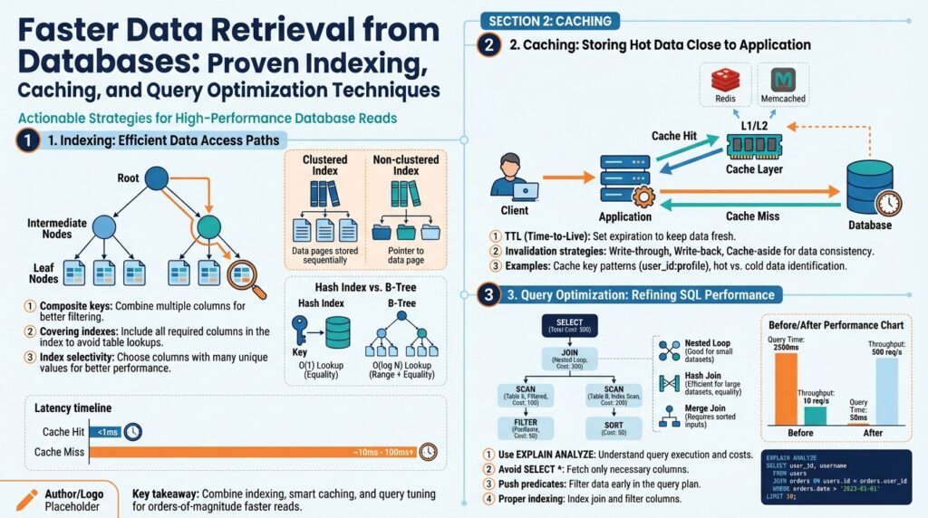
There are several index strategies to match application patterns: composite (multi-column) indexes for common multi-column filters, covering indexes that include all columns required by a query to enable index-only scans, partial indexes that index a subset of rows (e.g., WHERE active = true), and expression/index-on-computed-columns for queries that filter on transformations. Choose clustered indexes when the physical table ordering benefits range scans; otherwise prefer nonclustered indexes to minimize table layout constraints. Use parallel structure in planning: composite for combined predicates, partial for sparse heavy-use slices, expression for computed predicates.
Implementing indexes effectively is an iterative process: profile queries with EXPLAIN or EXPLAIN ANALYZE, add a targeted index, then validate plan changes and execution time on representative data. Track index usage statistics (pg_stat_user_indexes in PostgreSQL, sys.dm_db_index_usage_stats in SQL Server) and garbage-collect or drop unused indexes. Keep statistics current—run ANALYZE or equivalent—and schedule reindexing for heavily fragmented indexes. For large tables, create indexes concurrently where supported to avoid long locks and use sampling to estimate selectivity before committing to a global schema change.
Taken together, good indexing practices deliver fast, predictable reads while keeping write impact and storage costs manageable. Next, we’ll pair these indexing techniques with caching and query-level optimizations to address scenarios where even index-accelerated queries become a bottleneck. This combined approach helps you design systems that scale read latency, throughput, and operational simplicity in production.
Choosing the Right Index Types
Choosing the right index types starts with recognizing that not all indexes are equal and that index types shape both query latency and write cost. If you want predictable, low-latency lookups you must match index structure to access patterns—this is where index types become a design decision, not an afterthought. Building on the fundamentals we covered earlier, prioritize index choices that maximize selectivity for your hot paths while minimizing write amplification and storage overhead. We’ll focus on practical signals you can measure and concrete examples you can apply immediately.
Begin by characterizing your workload: are reads point lookups, range scans, frequent ORDER BYs, or heavy aggregations? This single question guides whether a hash or B-tree-like structure is appropriate, whether clustering the table helps range queries, and whether composite or covering index strategies will reduce I/O. Measure predicate selectivity and predicate frequency first—columns that are highly selective and used in WHERE, JOIN, or ORDER BY should be indexed before low-selectivity flags. For high-cardinality equality checks use hash or B-tree indexes for O(log n) lookups; for ranges and ordered scans prefer B-tree/clustered approaches.
How do you choose between a clustered index and a set of nonclustered/composite indexes? Choose a clustered index when your application performs many range scans on the same key (for example, time-series queries like SELECT * FROM events WHERE device_id = ? ORDER BY timestamp DESC LIMIT 100). Otherwise prefer nonclustered indexes to avoid rigid physical ordering that inflates update cost. For multi-column predicates, create a composite index that matches the common predicate order; for example:
CREATE INDEX idx_orders_customer_date ON orders(customer_id, created_at DESC) INCLUDE (total_amount);
This pattern serves three purposes: the leading column supports the equality filter, the second column accelerates ordered range scans, and the INCLUDE creates a covering index so the query can be served without touching the heap.
Use partial indexes and expression (computed) indexes when a small slice of rows drives most queries or when your predicates use transformations. Partial indexes restrict the index to rows that match a WHERE clause (e.g., WHERE status = ‘active’), dramatically reducing index size and write cost for sparse workloads. Expression indexes are invaluable when you filter on normalized or transformed values—index lower(email) for case-insensitive lookups rather than storing an extra column. Both strategies reduce maintenance overhead because they shrink the indexed set to what actually matters.
Always weigh the trade-offs: every additional index increases storage and write latency, and complex composite indexes can obscure optimizer choices if column order doesn’t match common predicates. Monitor index usage and write impact and prefer consolidated composite indexes over many single-column indexes when feasible. As we discussed earlier, track index hit rates and write throughput during representative traffic to validate that the chosen index types deliver real-world benefit rather than theoretical improvement.
Validate index selection with EXPLAIN ANALYZE and representative dataset tests before committing to schema changes in production. Simulate mixed workloads, check cardinality estimates, and test how planner statistics affect plan selection—if the planner misestimates selectivity, adding or refining an index type may not change performance. Create indexes concurrently where supported and iterate: add a targeted composite or partial index, benchmark, and then either promote it or roll it back. Taking this measured approach ensures your index types accelerate the actual queries that matter and leaves room to pair indexing with caching and query-level optimizations in the next step.
Designing Composite and Covering Indexes
Building on this foundation, the fastest wins often come from designing indexes that match how your queries actually filter, join, and sort. If you’re seeing many multi-column predicates or ordered range queries, a composite index combined with a covering strategy can convert expensive heap lookups into index-only scans and cut I/O dramatically. How do you choose column order and what should live in the index keys versus included columns? We’ll walk through concrete patterns you can apply to real query shapes and validation steps you should run before shipping changes to production.
Start with composite index fundamentals: a composite index stores multiple columns in a single sorted structure and obeys the leftmost-prefix rule, so the leading column determines which predicates the index can use. When you design a composite index, place columns used in equality filters first, followed by columns used for range scans or ordering; for example:
CREATE INDEX idx_orders_customer_status_date
  ON orders(customer_id, status, created_at DESC);
This index favors queries where you filter by customer_id and status and then page by created_at. Put the most selective equality predicates early when they substantially reduce candidate rows; this minimizes work for subsequent range or ORDER BY columns and helps the optimizer pick the index.
A covering index extends this idea by including non-key columns so the index contains every column the query needs, enabling an index-only scan that never touches the table heap. Use INCLUDE (PostgreSQL, SQL Server) or add appended key columns (depending on your DB) for large payloads you want to expose from the index without affecting sort order. For example:
CREATE INDEX idx_orders_cover
  ON orders(customer_id, status, created_at DESC)
  INCLUDE (total_amount, shipping_address_id);
With this pattern, a SELECT that projects total_amount and shipping_address_id can be satisfied entirely from the index, reducing random I/O and CPU.
Combine composite and covering strategies against concrete query shapes. If your hot path is SELECT total_amount FROM orders WHERE customer_id = ? AND status = ? ORDER BY created_at DESC LIMIT 10, the composite index above covers the equality and ordering while INCLUDE makes it index-only. In contrast, if you have queries that sometimes omit status, avoid an index that forces a poor leading-column choice; instead consider a smaller composite where customer_id is first and status is second, or add a partial index if status = ‘active’ drives most traffic. Always reason about selectivity, not just column cardinality—highly selective predicates give the optimizer confidence to use the index.
Be mindful of costs and common pitfalls. Every additional index increases storage and write latency—indexing many low-selectivity columns or adding large included payloads can slow inserts and updates. Database-specific behaviors matter: PostgreSQL uses a visibility map for index-only scans so frequent updates can prevent index-only plans, and some engines treat included columns differently for ordering. Validate with EXPLAIN ANALYZE on representative data and traffic; verify that the plan is an index-only scan and measure end-to-end latency under mixed workloads, not just isolated selects.
Operationalize your choices: create indexes concurrently when supported to avoid long locks, and combine partial or expression indexes with composite/covering techniques when a small slice of rows or a transformed predicate drives most queries. Track index usage metrics and stale statistics—if the optimizer misestimates cardinality, tuning statistics or rewriting predicates often yields bigger wins than another index. Weigh the marginal read latency improvement against write amplification and storage growth before promoting an index into production.
Taking a measured approach to composite and covering indexes turns indexing from a guess into a repeatable design pattern. When you match column order to predicate shape, include only the projection needed for index-only scans, and validate with real workloads, you reduce query latency while keeping write costs manageable. Next we’ll connect these index-level improvements to caching and query-level optimizations that further reduce tail latency and contention.
Query Analysis and EXPLAIN Usage
Building on this foundation, start every optimization cycle with disciplined query analysis and a targeted use of EXPLAIN so you know whether an index or rewrite will actually change the plan. EXPLAIN (the planner’s estimated plan) and EXPLAIN ANALYZE (the runtime-executed plan with timings) are the primary instruments we use to translate symptom-level latency into concrete action. Front-load EXPLAIN early in investigative workflows: run it on representative data and with realistic bind values so the plan you inspect matches production behavior. How do you decide which tool to run first and what to trust when they disagree?
Use EXPLAIN when you want a quick, zero-impact snapshot of the optimizer’s thinking; use EXPLAIN ANALYZE when you need to validate runtime performance. EXPLAIN returns estimated costs and cardinality estimates (the planner’s predicted row counts), while EXPLAIN ANALYZE executes the query and reports actual rows and execution time. Run EXPLAIN ANALYZE in a safe environment for heavy queries because it executes the statement—avoid running it on destructive DML in production without safeguards. For read-only investigation you can often pair EXPLAIN with connection-level settings (read-only, statement timeout) to reduce risk while capturing realistic plans.
When estimated rows diverge drastically from actual rows, you have a cardinality problem: the optimizer misestimates result sizes and pick an inefficient join order or access path. Start by comparing the planner’s “actual rows” to its “estimated rows” for each node; large underestimates commonly lead to nested-loop joins where a hash join would be faster or to choosing a seq scan over an otherwise usable index. Address this by refreshing statistics (ANALYZE), creating histogram-friendly statistics targets or extended statistics for correlated columns, and verifying data distributions—skew, NULL density, and outliers are frequent causes. If statistics and sampling settings look correct, the next step is rewriting predicates so the optimizer can reason about selectivity (for example, avoid wrapping column references in non-indexable functions).
Read plan nodes with a purpose: check scan types, join algorithms, and whether the plan becomes index-only or requires heap access. A Seq Scan indicates a full-table read; an Index Scan or Bitmap Heap Scan shows partial index use; an Index-Only Scan (when available) means the index contains all projected columns and the visibility map allowed skipping heap lookups. For joins, Nested Loop is great for small inner sets but catastrophic for large cross-products; Hash Join is usually better for large unordered inputs, and Merge Join excels when both inputs are pre-sorted. Also inspect loop counts and per-node timing and buffer hits—high buffer read/write activity at a node signals I/O hotspots even when CPU looks fine.
Translate plan observations into concrete changes and revalidate with EXPLAIN ANALYZE. If a join order is wrong, force less invasive fixes first: add a selective composite or covering index that supplies leading predicates, increase statistics targets, or rewrite queries (turn OR predicates into UNIONs that can use separate indexes, replace DISTINCT with EXISTS when deduplication is the bottleneck). Use optimizer hints only as a last resort and document them; hints can mask real underlying problems and diverge when data drifts. After each change, run EXPLAIN ANALYZE on representative workloads and measure end-to-end latency rather than micro-benchmarks—real traffic mixes reveal effects like visibility-map misses that synthetic runs miss.
Make query analysis part of your CI and regular maintenance cadence so plans don’t regress silently as data grows. Capture canonical EXPLAIN outputs for critical queries, track plan shape and timing across releases, and pair plan regression alerts with targeted actions (statistics refresh, index creation, or query rewrite). Taking this approach turns EXPLAIN from an occasional debugging tool into a repeatable diagnostic that pairs with indexing and caching to reduce tail latency and stabilize performance.
Caching Patterns: Cache-Aside and Write-Through
Building on this foundation, the next pragmatic lever to reduce read latency is an in-memory cache that sits between your application and the indexed data store. A cache short-circuits repeated index lookups for hot keys and reduces I/O, cutting tail latency when your database is otherwise well-indexed but still under heavy read pressure. We’ve seen index tuning convert full-table scans into index-only scans; a cache takes that a step further by avoiding even the index lookup for very hot objects. How do you pick the right caching approach for your hot paths?
The most common application-driven approach is the cache-aside pattern, where your code explicitly checks the cache before hitting the database and populates the cache on a miss. With cache-aside you control population and eviction: on a read miss you read from the DB, then write the result into the cache with an appropriate TTL or version token. This pattern fits read-heavy endpoints with complex write semantics because writes update the database first and then invalidate or refresh the cached value; you avoid write amplification at the cache but accept a small window of staleness unless you aggressively invalidated. Cache-aside also gives you precise control for partial-cache scenarios—when only a small slice of keys is hot relative to overall data size.
The write-through approach takes the opposite operational stance: every write goes to the cache and the cache synchronously writes through to the backing store, ensuring the cache is always warm for reads. This pattern simplifies read-after-write consistency because subsequent reads can rely on the cache reflecting the latest committed state, and it reduces cache-miss spikes during bursts. The trade-off is higher write latency and potential write amplification: each application write likely touches two systems and requires error handling for cache or DB failures. Use write-through when you need deterministic cache-coherency for critical entities and when write rates are moderate enough that the extra latency and throughput cost are acceptable.
Comparing the two, think of cache-aside as giving you control and lower write overhead, while write-through gives you simpler consistency at the cost of write performance and complexity in failure modes. Cache-aside is often better for high-cardinality keys where only a small percentage is hot and where you already manage complex transactional writes; write-through is attractive for small, bounded datasets where reads must immediately reflect writes. Consider real-world examples: user profile reads that tolerate brief staleness pair well with cache-aside, whereas a payment authorization state machine that must be consistent across reads and writes might justify write-through. Which pattern you choose should be driven by your read/write ratio, acceptable staleness, and operational tolerance for extra write latency.
In practice you must also solve engineering details regardless of pattern: design stable cache keys that reflect the indexable identity (for example, user:{id}:profile), choose sensible TTLs and use versioning or Last-Write-Wins tokens for optimistic validation, and implement stampede protection for cold-cache misses. Defend against race conditions with double-checked locking or singleflight mechanisms so multiple requests don’t concurrently repopulate the same key. Instrument cache hit ratio, miss latency, eviction rates, and write amplification metrics; these telemetry signals tell you when an index or a cache change is actually improving end-to-end latency rather than masking a deeper database contention.
Building on our earlier discussion of indexing and EXPLAIN, cache strategies should complement—not replace—good index design and query rewrites. Use caching for point lookup hot paths that competitors’ indexes already accelerate; avoid caching large scan results that should instead be optimized with covering indexes or pagination. Validate changes with representative workloads: measure end-to-end request latency under mixed read/write traffic, compare index-only scans against cached responses, and watch for plan regressions as data shapes change. With careful key design, eviction policy, and instrumentation, these caching patterns become repeatable tools that reduce tail latency and keep your indexed database serving efficiently as traffic scales.
Partitioning, Sharding, and Scaling Strategies
Building on this foundation, when your single-node indexes and cache layers stop delivering predictable latency, you need to rethink data placement: partitioning, sharding, and other scale approaches become operational levers rather than theoretical options. If your read or write throughput grows past what a single instance can sustain, you must choose how to split data so queries remain index-friendly and I/O stays local. How do you pick between database-level partitioning and application-level sharding, and when is it better to scale horizontally versus vertically?
Start by separating concepts: partitioning is an internal table organization that keeps related rows contiguous (helping range scans and pruning), while sharding distributes data across distinct database instances so you scale storage, CPU, and I/O horizontally. Use partitioning for large tables where predicates naturally slice data—time-series events or archive tables are classic fits—because the planner can prune entire partitions and reduce IO. For example, in PostgreSQL you might write:
CREATE TABLE events (id bigint, device_id uuid, created_at timestamptz, payload jsonb)
  PARTITION BY RANGE (created_at);
CREATE TABLE events_2025_01 PARTITION OF events
  FOR VALUES FROM ('2025-01-01') TO ('2025-02-01');
Shard key selection is the most consequential decision you’ll make because it shapes query locality, hotspot risk, and resharding difficulty. Choose a shard key that aligns with your dominant access pattern: user_id works well for per-user workloads, tenant_id for multi-tenant isolation, and order_id is useful when writes and reads are co-located to orders. Avoid monotonically increasing keys (timestamps, sequential IDs) as primary shard keys because they concentrate writes; prefer hash-based partitioning or use composite keys that mix entropy (tenant_id || user_id). When you anticipate uneven distribution or bursts, use virtual nodes or consistent hashing to rebalance without moving large contiguous ranges.
Plan for resharding from day one because data growth and traffic patterns change. Implement one of three pragmatic approaches: online rehashing with routing-layer remapping and background backfill, dual-writes plus a cutover once backfill completes, or use a lookup table that maps logical keys to physical shards and can be updated atomically. Each approach trades complexity against downtime and data duplication: background backfill avoids downtime but requires careful idempotency and verification, while a controlled cutover simplifies correctness but costs a maintenance window. Instrument end-to-end checksums, row counts, and query-sample parity during resharding so you can validate correctness before redirecting live traffic.
Combine partitioning and sharding with indexing and caching choices you already made: local indexes on each shard reduce intra-shard I/O, but global secondary indexes become expensive and often require a separate index service or a metadata layer. For read-heavy hot keys, keep cache-aside or write-through caches at the application edge so you avoid cross-shard fan-out for point lookups; for analytic queries spanning shards, push down filters to each shard and aggregate results rather than shipping all data. Be explicit about consistency boundaries—eventual consistency across shards is acceptable for many read caches, but transactional guarantees spanning shards demand two-phase commit or distributed transaction patterns, which increase latency and operational overhead.
Operational scaling involves more than splitting data: add read replicas to absorb read traffic, monitor replication lag closely, and use connection routing or proxies to send writes to primaries and reads to replicas. Measure saturation metrics—CPU, IOPS, lock contention, and tail latency—so you scale when resource utilization, not just traffic volume, dictates it. Automate alerts on plan regressions and shard hotspots; when a shard approaches its resource limits, act early with resharding or by moving heavy tenants off to isolated instances.
Taken together, a pragmatic strategy blends partitioning for planner efficiency, sharding for horizontal capacity, and operational controls for resilience. We should design shard keys that match query locality, plan online resharding paths, and keep caching and indexing aligned with the distribution model so queries stay fast as we scale. Next we’ll connect these distribution patterns to query-level optimizations and cache strategies so you can reduce cross-shard cost and stabilize tail latency.