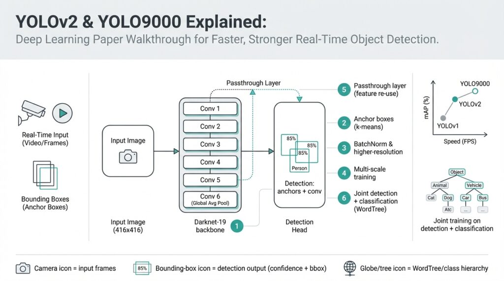
YOLOv2 and YOLO9000: Paper Overview
Imagine you’ve been playing with toy object detectors and you want something that runs fast enough to inspect live video while staying accurate enough to trust. In 2016–2017 two closely related advances — YOLOv2 and YOLO9000 — pushed real-time object detection (detecting and labeling objects in images or video frames fast enough for live use) forward by redesigning both the model and the training recipe. Building on the idea that speed matters as much as accuracy, these papers ask a clear question: how do we get a single neural network to detect many kinds of objects quickly and reliably?
At the heart of the story is a shift in how the network thinks about boxes and classes. YOLOv2 replaces older ad-hoc box regressors with anchor boxes — pre-defined box shapes that the network tweaks to match objects — which makes predicting varied object sizes more stable. The authors also borrow practical tricks: batch normalization (a method that normalizes layer inputs to stabilize and speed training), high-resolution classifier fine-tuning (pretraining on larger images before detector training), and a slimmer, faster backbone network called Darknet-19 (a convolutional neural network architecture optimized for speed). These changes read like tuning an engine: each small adjustment makes the model run smoother and push better performance.
Let’s tell the architecture’s next chapter as a short scene. First, the image passes through convolutional layers that learn visual features (edges, textures, shapes) at increasing levels of abstraction. Then the network predicts, at several spatial locations, pairs of numbers that describe bounding boxes and a set of class probabilities for each anchor box. To make those anchor boxes actually match the dataset, YOLOv2 uses k-means clustering (a simple method that groups similar box sizes together) on ground-truth boxes to pick good box priors, so the model starts with box shapes that reflect the data it will see in the wild.
YOLO9000 takes the exploration further by asking, what if we want to detect thousands of categories but only have bounding boxes for a few? The clever answer is joint training on detection and classification datasets: the model learns to detect objects from labeled detection datasets (which have box annotations) while simultaneously learning a large vocabulary of classes from classification datasets like ImageNet. To reconcile different label sets, the authors build a hierarchical label map (WordTree) that organizes classes by semantic relationships — think of it like a family tree for object names — letting the model reason that “German shepherd” is a kind of “dog,” so learning dog features helps even when a specific dog breed lacks boxes.
How does this feel in practice? Picture feeding a street scene into the network: features flow through Darknet-19, anchor box offsets and objectness scores are predicted at each grid cell, class probabilities are attached, and non-max suppression (a simple filter that removes overlapping duplicate detections) cleans up the final list. The training balances multiple losses — location, confidence (objectness), and classification — so the network learns where objects are and what they are at the same time. That joint learning is exactly why YOLO9000 can output labels for many classes without having seen box annotations for each one: it has learned class concepts and how to localize objects as separate but compatible skills.
We should be honest about trade-offs: these papers favor speed, so they accept some accuracy compromises compared with slower, two-stage detectors (two-stage detectors first propose regions, then classify them). Accuracy is measured with mAP, mean average precision (a summary number that captures both how often detections are correct and how precisely boxes fit). YOLOv2 improves mAP substantially over the original YOLO while keeping frame rates high, and YOLO9000 demonstrates the feasibility of large-vocabulary detection by showing reasonable performance on thousands of classes.
Now that the main ideas and practical tricks are clear, the natural next step is to open the model internals and walk through training and implementation details so you can run and adapt these networks yourself. In the following section we’ll take that journey together: we’ll set up the Darknet codebase, inspect model files, and run small experiments so you can feel how these design choices change results in the real world.
Darknet-19 Backbone: Architecture and Design
Imagine you’re tuning a model for live video: you need Darknet-19, the backbone in YOLOv2, to be both quick and capable so real-time object detection doesn’t feel like a trade-off between speed and usefulness. You’re standing at the crossroads of accuracy and latency, wondering how a network can stay slim yet learn features rich enough to localize and classify objects. How does this compact design keep accuracy while running at frame rates suitable for real-time object detection? Let’s walk through the architecture like we’re unpacking a compact toolkit built for speed.
The high-level layout reads like a short, efficient novel: nineteen convolutional layers interleaved with five downsampling steps (max-pooling), capped by a few 1×1 convolutions that act as a bridge to the detection head. This structure replaces the bulky fully-connected layers used in older classifiers with only convolutional operations, which preserves spatial information and reduces parameters — important when you want a backbone that feeds meaningful feature maps into the detector without slowing everything down. Each convolution is followed by batch normalization and a leaky ReLU activation, a small but crucial pattern that repeats throughout the network.
Think of the 3×3 convolutional layers as the core recipe: stacking small kernels lets the network build larger receptive fields step by step, like layering flavors in a stew. Two stacked 3×3 convolutions capture the context of a 5×5 region while keeping parameters lower and computation more cache-friendly than a single large filter. Scattered among them are 1×1 convolutions — these are the kitchen scalpel: they mix channels, squeeze and expand feature maps, and cut down on parameter count so we can afford deeper representations without a huge computational bill.
A quiet hero in the design is batch normalization. Placed after almost every convolution, it standardizes the output distributions so training runs faster and more stably; that stability lets us use more aggressive learning rates and get to a good model quicker. Paired with leaky ReLU activations (which allow a small gradient when units are negative), these choices make Darknet-19 resilient during optimization: fewer dead neurons, steadier gradients, and a backbone you can train from scratch or fine-tune for detection without endless hyperparameter tinkering.
Spatial downsampling in the network is handled by a sequence of pooling operations that progressively reduce width and height while increasing channel richness — the classic funnel that trades spatial resolution for semantic abstraction. But YOLOv2 knew we still needed some of the finer-grained texture for small objects, so the design borrows a passthrough (or reorg) mechanism to pull higher-resolution features from an earlier layer into the detection stage. That shortcut is like folding a fine-print map into the main atlas: it gives the detector local detail and global context at once, improving localization for smaller, tougher targets.
All these choices are about efficiency trade-offs more than clever tricks for trickiness’s sake. By favoring 3×3 and 1×1 convolutions, removing dense heads, and adding normalization and light activations, Darknet-19 keeps parameter counts and FLOPs down so you get good accuracy per millisecond. In practice this means you can run the backbone on constrained hardware or push higher frame rates while still producing feature maps rich enough for anchor-box-based predictions and class probabilities.
Building on this understanding of the backbone, the next step is practical: mapping these architectural pieces to model files and configuration blocks so we can run experiments. With the intuition in place — why 3×3 stacks, why 1×1 bottlenecks, why batch norm and passthroughs — you’ll recognize each layer when we inspect the Darknet config and tweak it for your own datasets and speed targets.
Anchor Boxes via K-means Dimension Clustering
Imagine you’ve built a detector and the boxes it predicts look all over the place: some are too tall, others too wide, and the network seems to struggle to settle on common object shapes. Right away we reach for anchor boxes and k-means clustering to give the model a sensible starting point; anchor boxes are pre-defined box shapes the network can tweak, and k-means clustering is a way to group the dataset’s box sizes so those pre-defined shapes match reality. Front-loading good anchor box priors makes training smoother because the network learns offsets from realistic templates instead of inventing shapes from scratch.
We first meet anchor boxes as helpers, not replacements: an anchor box is a rectangle prior—defined by width and height—that sits at each grid cell and says, “Start here and nudge me.” This reduces the regression problem: instead of predicting absolute coordinates for every object, the network predicts adjustments (offsets) relative to these priors. By defining anchor boxes that reflect the common aspect ratios and scales in your images, you free the model to focus on refining positions and confidences, which usually speeds convergence and improves localization.
So how do we pick those priors? That’s where k-means clustering on box dimensions enters the story. K-means clustering is a simple algorithm that groups similar items together; for boxes we cluster width–height pairs so boxes with similar shapes end up in the same group. YOLOv2 uses a distance based on Intersection over Union (IoU)—IoU measures overlap between two boxes—to cluster by shape similarity rather than raw Euclidean distance. Defining the distance as 1 − IoU makes the clusters reflect how well a proposed prior would overlap actual boxes, which is what matters for detection.
Let’s walk through the practical steps like a short recipe: extract every ground-truth box’s width and height and normalize them by the image dimensions so sizes are comparable across different images. Choose a k (a handful of clusters; YOLOv2 used five) and run k-means with the IoU-based distance to find k centroids—those centroids become your anchor box priors. Ask yourself: “How do I choose k?” The answer is empirical: more clusters can match the data more closely but add complexity to prediction; evaluate average IoU of clusters with ground truth and pick a k that balances coverage and simplicity.
Why does this work better than hand-picked sizes? Think of it like buying luggage: you could guess which suitcase sizes you need, or you could measure what you actually carry and buy a set that fits. K-means-derived anchor boxes mirror the dataset’s shape distribution, which reduces large systematic errors (for example, a dataset dominated by tall pedestrians won’t be forced into wide car-like priors). Practically, these data-driven priors improve the starting point for the network’s box regressors, reduce training instability, and often yield higher mAP because the model learns to refine realistic templates rather than learn shape from zero.
There are a few actionable tips we like to follow. Always normalize widths and heights by image size before clustering, test several k values and compare average IoU scores, and map the resulting centroids to the detector’s stride or grid so they align with the prediction cells. If your dataset changes (new camera, different aspect ratios), rerun the clustering—good anchor boxes are specific to your data distribution. With anchor box priors tuned this way, the detector’s job becomes clearer and faster; next we’ll look at how those priors are used by the detection head so predictions turn into clean, confident bounding boxes.
Passthrough Layer and Multi-scale Training
Imagine you’re staring at detections that look confident but miss the small things you care about—the phone on a table, the distant traffic sign, the bird in the corner. We’ve seen that problem before, and one of the tidy engineering answers in YOLOv2 is the passthrough layer: a bridge that brings higher-resolution detail from an earlier layer into the final detection stage. A passthrough layer (sometimes called a reorg connection) lets the network keep both the big-picture context and the fine-grained texture, which matters when tiny objects sit inside large scenes.
First, let’s meet the cast of characters. A feature map is the grid of values produced by a convolutional layer; channels are the separate slices of that grid that respond to different visual patterns (think of them like color channels, but learned). The passthrough layer takes a higher-resolution feature map—where spatial detail is still rich—and reorganizes its layout so it can be concatenated with the deeper, lower-resolution feature map used for detection. This spatial-to-depth reorg converts nearby pixels into extra channels so the two maps line up spatially and the detector sees more local detail without losing semantic depth.
Here’s a concrete picture of what happens under the hood: imagine a shallow layer with a 26×26 feature map and a deeper detection layer at 13×13. The reorg operation collects each 2×2 patch in the 26×26 map and stacks those four values into the channel dimension of a 13×13 map (that’s spatial-to-depth). Once reshaped, the higher-resolution information and the deeper features share the same 13×13 grid and can be concatenated along channels. The result is a richer detection tensor that combines fine texture and high-level context in a single place.
Why does this help small object detection? Small objects often vanish as the network down-samples; their signal gets averaged away in deeper layers. By folding earlier, higher-resolution cues into the detection layer, the model preserves local edge and texture information that anchors and bounding-box regressors can use. Put simply: the passthrough gives the detector the “zoomed-in” clues it lost while still benefiting from the deeper layer’s semantic understanding.
Now let’s turn to training the network to handle different image sizes: multi-scale training. Multi-scale training is the practice of varying the input image resolution during training so the model learns to detect across a range of sizes and densities. Because the backbone is fully convolutional—meaning it can accept different input widths and heights without changing its weights—we can randomly change the training image size every few iterations and force the detector to adapt its internal representations to multiple scales.
In practice, multi-scale training works by selecting image sizes that are multiples of the network’s downsampling stride (for YOLO-style models this is commonly 32) and resizing the input accordingly during training. For example, training might randomly pick dimensions between 320 and 608 pixels (in steps of 32) so the model sees small, medium, and large views. That variability teaches the network to be robust: at inference you then choose a single size that balances speed and accuracy for your application, but the model itself will generalize better to different camera resolutions.
There are trade-offs to keep in mind. Larger inference sizes usually improve detection for small objects at the cost of latency and compute; smaller sizes speed up real-time applications but can miss fine details. Using both the passthrough layer and multi-scale training together gives you flexibility: the passthrough preserves detail within the model, and multi-scale training ensures the model learns to use that detail across a range of input resolutions. If you need a practical rule: train with multi-scale, use passthrough for small-object-heavy datasets, and pick your inference size based on the hardware you have.
Before we move on to running experiments, remember the actionable takeaways: the passthrough/reorg connection preserves higher-resolution cues by reshaping spatial information into channels, improving small object localization; multi-scale training exposes the model to a spectrum of input sizes so it adapts gracefully; and at inference you pick the size that fits your speed/accuracy budget. With those levers in your toolkit, we can now test how different sizes and reorg placements change real results on your own dataset.
Joint Training with WordTree Hierarchical Classes
Imagine you want a fast object detector that knows thousands of names but you only have bounding boxes for a handful of them — this is exactly the problem YOLO9000 set out to solve with joint training and a clever label hierarchy called WordTree. WordTree is a hierarchical label map that groups related class names by meaning (a “family tree” for labels), and joint training means we teach the network from both detection datasets (images with bounding boxes) and classification datasets (images labeled with a single class) at the same time. Right away we see the payoff: hierarchical classes let the model share visual knowledge across similar categories, so learning about a general concept like “dog” helps it recognize finer breeds even when breed boxes aren’t available. This idea rewrites the vocabulary problem in object detection into a transfer-learning story.
Start by meeting the two datasets as characters in the plot. A detection dataset is a collection of images where each object of interest has a bounding box and a class label; a classification dataset is a larger set of images labeled at image level (what’s in the photo) but usually lacks boxes. The mismatch is natural: detection labels are expensive to collect, classification labels are cheaper and abundant. Joint training stitches these two sources together so the detector learns localization from boxed examples while absorbing a much wider semantic vocabulary from classification images, expanding what it can name without needing box annotations for every class.
Next, let’s follow how the WordTree plays its role. Think of hierarchical classes as an organized filing cabinet: broad categories sit near the root and specific subclasses hang off branches. WordTree maps each class label onto that cabinet so labels share ancestors — “German shepherd” and “beagle” live under “dog,” which in turn lives under “animal.” During training, the network learns to predict probabilities along that path, letting general visual features (fur, snout, four legs) reinforce many fine-grained labels. By treating labels as related rather than independent, WordTree reduces confusion between synonyms and supports transfer from coarse labels to fine-grained ones.
So how does the model actually learn from both kinds of data? The network is trained in a multi-task way: on detection images we optimize localization (boxes) and class predictions, and on classification images we optimize class prediction across the WordTree nodes without a box loss. “Loss” here means the training signal that measures how wrong the model is and tells it how to update weights. Because class labels are organized hierarchically, classification examples update shared ancestors and leaf nodes in the tree, while detection examples anchor those learned concepts to spatial locations. In practice this alternating or mixed-batch training lets a single detector internalize both where objects are and a much larger set of what they might be.
Imagine we only have boxes labeled “dog” in the detection set but ImageNet-style classification data tells us “German shepherd” exists. What do we get? The detector learns to localize dogs from the boxed data and, through WordTree, learns the visual signals that distinguish German shepherds from other dogs from the classification data. At inference the network can output “German shepherd” for a detected dog because it has both the localization skill and the semantic knowledge; the hierarchy made that hand-off possible. How do you handle ambiguous or overlapping labels? The hierarchy helps: the model can fall back to a parent label (like “dog”) when a finer-grained prediction is uncertain.
There are trade-offs and practical tips to keep in mind. Joint training increases the demands on model capacity and careful balance: classification datasets can overwhelm rare detection labels if you don’t weight losses or sample batches thoughtfully. Noisy or mismatched taxonomies are another hazard — your WordTree must align names and synonyms across datasets, or you’ll teach the model confusing signals. For best results, curate a clean mapping between detection and classification labels, experiment with loss weights, and monitor errors at different tree levels so we know whether the model is learning localization, semantics, or both.
Building on the architectural pieces we’ve already explored, the next step is practical: assemble a WordTree mapping, prepare mixed training batches that include both boxed and unboxed images, and tune the loss balance so localization and semantics rise together. When done well, this joint-training + WordTree approach turns a detector into a large-vocabulary labeler that can localize many more classes than you could box-annotate alone — a powerful way to scale object detection without a proportional increase in annotation cost.
Practical Implementation, Training, and Inference Tips
If you’ve followed the earlier walk-through of YOLOv2 and YOLO9000 for real-time object detection, you’re probably itching to run a model and see how those design choices behave on real images. In practice, implementing these networks is less about mystery and more about a careful recipe: prepare your data, pick sensible anchors and training hyperparameters, use multi-scale tricks, and tune inference thresholds. We’ll walk through each of those steps together so you can avoid common pitfalls and get dependable results faster.
First, let’s talk data preparation because good inputs make training feel effortless. Your dataset should have consistent image formats and correct labels — a bounding box is simply four numbers (x, y, width, height) that localize an object. Normalize box widths and heights by image size before you run k-means for anchor boxes so those priors reflect the distribution of shapes in your photos. If you mix sources, align class names (the WordTree mapping you read about earlier is useful) so the model doesn’t learn conflicting labels; think of this as naming consistency in a cookbook so every ingredient is the same across recipes.
Next comes training setup: this is where you balance speed and stability. Batch size is the number of images processed together and affects gradient noise; larger batches give steadier gradients but require more memory. Learning rate controls how large each weight update is—start with a conservative schedule and use warm-up if you’re training from scratch. Fine-tune means starting from a pretrained classifier (like Darknet-19 pretrained on ImageNet) and then training the detector; this usually shortens convergence and stabilizes learning. Monitor training losses separately for localization (how well boxes fit) and classification so you can spot which part needs attention.
How do you choose anchor boxes and loss weights in practice? Run k-means with an IoU-based distance (IoU, or Intersection over Union, measures overlap between two boxes) on your ground-truth boxes to get 4–6 priors that match your data. Map those priors to the network stride so each anchor aligns with a grid cell. If small objects dominate, increase the number of smaller priors or add the passthrough connection we discussed earlier. Balance your loss terms by scaling the box regression loss relative to classification—if the model finds boxes but mislabels them, raise the classification weight; if boxes are noisy, raise the localization weight.
Multi-scale training and augmentation are the secret sauce for robustness. Randomly vary input size every few iterations (sizes should be multiples of the network’s stride) so the model learns to handle different camera resolutions. Use standard augmentations—random flipping, color jitter, small translations—but avoid extreme distortions that break object geometry. At inference time pick the largest input size your hardware supports for best accuracy on small objects, and reduce size when you need throughput for real-time video.
Inference tuning is a practical art: non-max suppression (NMS) removes overlapping detections so you don’t see duplicate boxes, and a confidence threshold filters out weak predictions. NMS works by keeping the highest-confidence box and removing others with IoU above a threshold; sweep that IoU and confidence threshold on a validation set to find the sweet spot. If you see many false positives, raise the confidence threshold; if you miss objects, lower it or reduce the NMS IoU so boxes aren’t suppressed too aggressively.
When experiments fail, debug methodically. Visualize predicted anchors and ground-truth boxes to check alignment, inspect per-class precision/recall to find label imbalances, and try freezing pretrained layers if gradients are unstable. Small, iterative changes—recomputing anchors, adjusting learning-rate schedules, or reweighting loss terms—usually lead to big improvements. Building on what we covered earlier about the architecture and joint training, these hands-on tips will help you turn YOLOv2/YOLO9000 designs into reliable, fast object detection systems you can trust on real video streams.